Congaree Big Trees - Sufficiently Minimal

Introduction

This post is an expansion on a term project completed for SCHC 312 at the University of South Carolina during the Fall 2016 semester taught by Dr. John Grego. The project involved validating a big-tree database and then subsequently mapping the results. Ultimately though, it left us with more questions than answers.

The Congaree National Park is South Carolina’s only National Park. It is known most prominently for its abundance of massive trees that are also some of the oldest preserved individuals of their species in any floodplain ecosystem. There are a few environmental and historical reasons that have allowed for this. A temperate climate and nutrient rich soil provide an environment that is conducive to growth, and the historical inaccessibility of the park to loggers due to frequent floods from the Congaree River and an oppressive mosquito presence have preserved some of the park’s most impressive specimens.

Such favorable conditions have earned the Congaree distinction for its concentration of champion trees, or a tree judged by the National Parks Service for being the most impressive of its species according to a standardized criteria.

While champion trees serve as a major attraction for the Congaree National Park, identifying and regularly verifying the park’s resident champions is no easy task. Like any other tree, a champion is prone to falling over during storms (or in some cases, growing significantly since the last survey), so the park’s champion tree database must be regularly updated. The park’s Frank Henning has curated a sizable database, that is the product of the efforts of volunteers, researches, students, and park staff.

At the end of the semester, we had created a map of the trees in this database using Google Fusion Tables. We had chosen to use Fusion Tables because our date were already in a Google Sheet, but I had always intended to reproduce the map in R and do some further analysis.

Champion Tree Mapping

Setup

Since I want to retain the interactive functionality of the original map, I’ll use the leaflet package for mapping.

First, I’ll read in the champion tree data set and perform some minor cleaning and manipulation steps (the file is already relatively easy to work with).

cong <- read_csv("https://raw.githubusercontent.com/carter-allen/CongareeTrees/master/cong_trees.csv") %>% 
  mutate(lat = as.numeric(Latitude_NAD83),
         lon = as.numeric(Longitude_NAD83),
         type = identify_types(Common_Nam),
         Circumfere = as.numeric(Circumfere))

Note that the identify_types() function is defined (but not shown for aesthetic purposes) in this document to take in the common name of a certain tree and return a simple category that will be used for mapping. To illustrate:

identify_types(c("Red oak","Baldcypress","Loblolly Pine","A mystery tree"))

## [1] "oak"     "cypress" "pine"    "other"

The next step was to find images online to serve as icons for leaflet::addMarkers(). I wanted each tree in the data set to be identified by a small pictoral representation of that tree. However, since there are 73 unique values in the Common_Nam column, (check with cong %>% select(Common_Nam) %>% unique()), this seemed a bit impracticle. The identify_types() function grouped these trees into the following categories.

cong %>%
  group_by(type) %>%
  summarize(n = n()) %>%
  arrange(desc(n))

## # A tibble: 5 x 2
##   type         n
##   <chr>    <int>
## 1 other      132
## 2 oak         54
## 3 pine        28
## 4 cypress     16
## 5 sweetgum    14

So, I ended up finding 5 stock photos of trees on line to represent the 5 types of trees present.

Map

Now we are ready to map!

leaflet(data = cong) %>% 
  addTiles() %>% 
  addMarkers(~lon,~lat, 
             icon = ~tree_icons[type],
             label = ~htmlEscape(paste("A",Height,"feet tall,",
                                       Circumfere,"in. thick",
                                       Common_Nam)))

Other Visualizations

Below are two additional plots that summarize this data set nicely.

cong %>%
  filter(Height > 0 & Spread > 0 & Circumfere > 0) %>%
  group_by(Common_Nam) %>%
  summarize(n = n(),
            avg_ht = mean(Height)) %>%
  top_n(10,n) %>%
  ungroup() %>%
  ggplot(aes(x = reorder(Common_Nam,-n),
             y = avg_ht,
             size = n)) +
  geom_point() +
  theme(panel.background = element_rect(fill = "white"),
        text = element_text(family = "serif"),
        axis.text.x = element_text(angle = 35)) +
  xlab("Common Name") + 
  ylab("Average Height (ft.)") +
  ggtitle("Average Height of Top-10 Most Frequent Species") +
  labs(subtitle = "More than 10 are included because of ties")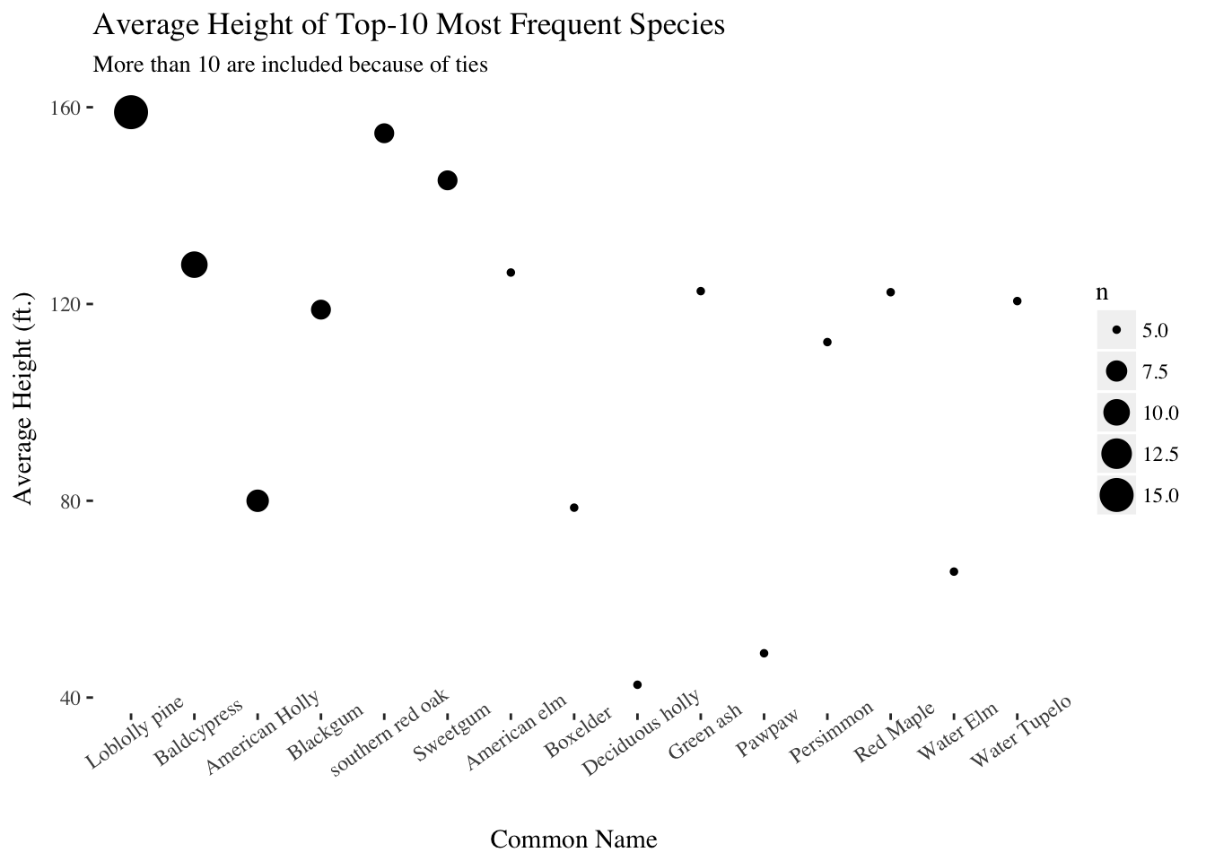

It is astonishing that the average height of champion-caliber loblolly pines in the park is around 160 ft.

cong %>%
  filter(Height > 0 & Spread > 0 & Circumfere > 0) %>%
  ggplot(aes(x = Circumfere, y = Height, size = Spread,color = type)) +
  geom_point(alpha = 0.85) + 
  scale_color_brewer(palette = "Greens") +
  theme(panel.background = element_rect(fill = "white"),
        text = element_text(family = "serif")) +
  xlab("Circumference in inches") +
  ylab("Height in feet") +
  ggtitle("Height vs. Circumference of Congaree Big Trees") +
  labs(subtitle = "Points colored by tree type and sized by canopy spread (ft.)")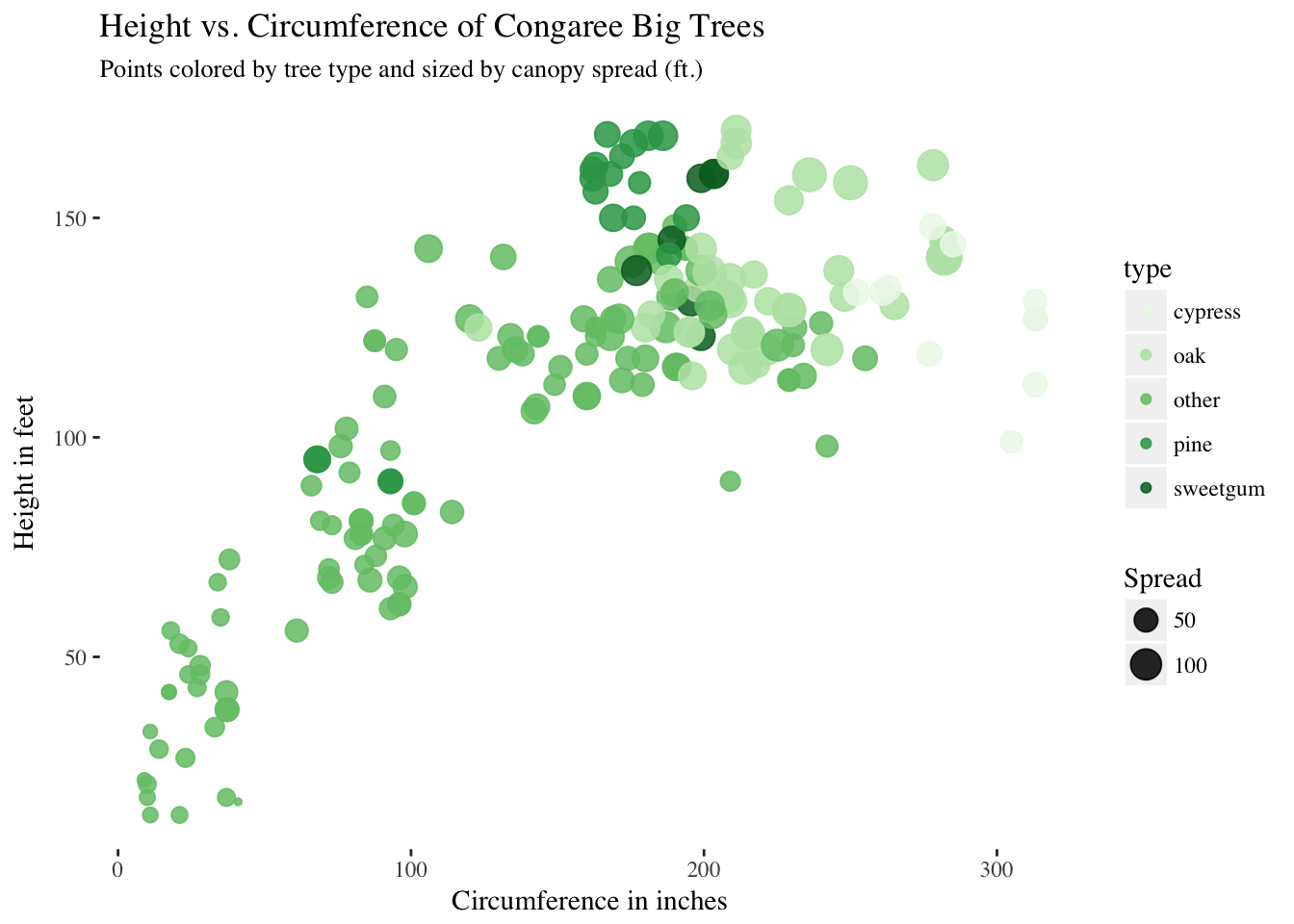

We can see a clear relationship between Height and Circumference, as expected, and can also recognize similarly clustered groups.

Concluding Remarks

I feel that the three vizualization techniques presented here adequately summarize the information contained in the big tree database. It is interesting to see clusters of tree types in both the map and the last figure.