This analysis looks at data on the sightings 🔭 of unidentified flying objects 🛸 covering 1904-2014. The data set contains 80332 sightings from countries all over the world with dates, times, locations and descriptions, among other features. The data is provided by the National UFO Reporting Center (NUFORC) by way of Kaggle.

Introduction to the Data
There are two data sets available on Kaggle, one titled complete.csv and one titled scrubbed.csv. The scrubbed data set will be used here as it eliminates missing or incomplete reports. The scrubbed data set can be downloaded here.
Reading scrubbed.csv
# read scrubbed.csv
library(tidyverse)
ufos <- read_csv("scrubbed.csv")
readr has some trouble with the scrubbed.csv file using that above code (I suppressed the warning messages for aesthetic purposes). Let’s try to get an idea of where the problems came from though.
probs <- problems(ufos)
probs
## # A tibble: 266 x 5
## row col expected actual file
## <int> <chr> <chr> <chr> <chr>
## 1 1606 duration (seconds) no trailing characters .5 'scrubbed.csv'
## 2 1653 duration (seconds) no trailing characters .5 'scrubbed.csv'
## 3 1660 duration (seconds) no trailing characters .1 'scrubbed.csv'
## 4 1683 duration (seconds) no trailing characters .5 'scrubbed.csv'
## 5 2039 duration (seconds) no trailing characters .05 'scrubbed.csv'
## 6 2275 duration (seconds) no trailing characters .5 'scrubbed.csv'
## 7 2336 duration (seconds) no trailing characters .5 'scrubbed.csv'
## 8 2344 duration (seconds) no trailing characters .2 'scrubbed.csv'
## 9 2431 duration (seconds) no trailing characters .1 'scrubbed.csv'
## 10 2618 duration (seconds) no trailing characters .5 'scrubbed.csv'
## # ... with 256 more rowsSo there were 266 problems reading the data in. These first ten are all the same kind of problem though - readr was thrown off by a decimal in the duration (seconds) column. Let’s see what other kinds of problems came up.
probs %>%
  select(col,expected) %>%
  unique()
## # A tibble: 2 x 2
## col expected
## <chr> <chr>
## 1 duration (seconds) no trailing characters
## 2 latitude no trailing charactersSo we had two distinct instances of the same problem. Some in the duration (seconds) column and some in the latitude column.
probs %>% filter(col == 'latitude')## # A tibble: 1 x 5
## row col expected actual file
## <int> <chr> <chr> <chr> <chr>
## 1 43783 latitude no trailing characters q.200088 'scrubbed.csv'I think this is just a data entry error. Perhaps \(q.200088\) is supposed to be \(20.00880\)? I’d like to not make any assumptions, and since this is only one row I feel safe just dropping it.
ufos <- ufos %>%
  filter(row_number(latitude) != 43783)
The only parsing problem left now is the duration (seconds) column. Unfortunately the duration (seconds) and duration (hours/min) are each a total mess and not really of interest here, so we’ll proceed without them 👋.
ufos <- ufos %>%
  select(-c(`duration (seconds)`,
            `duration (hours/min)`))
Further wrangling
I don’t care too much about the information contained in the date posted column so that will be dropped. It’ll also probably be helpful to parse that datetime column now.
ufos <- ufos %>%
  select(-`date posted`) %>%
  separate(datetime, c("date","time"), sep = " ")  %>%
  mutate(date = parse_date(date, "%m/%d/%Y")) %>%
  separate(time,c("hr","min"),sep = ":") %>%
  mutate(hr = parse_number(hr))
Visualization
Now for the fun part 📈! I will use the ggmap,maps, and mapsdata packages to plot UFO sightings around the world. The fist step will be to load the packages and define some map objects with the map_data() function.
library(ggmap)
library(maps)
library(mapdata)

world <- map_data("world")
n_america <- map_data("world",c("usa","Canada","Mexico"))
states <- map_data("state")
Now, since I plan to try out a few different maps, I am going to write a function called plot_ufos() that contains the code for formatting a nice map. The function will take in parameters for a map object (created above), UFO data (the full set or just a subset),the x-axis limits (longitude limits), y-axis limits (latitude limits), and a title for the plot. Below is the function definition.
plot_ufos <- function(map_object,ufo_data,x_scales,y_scales,title)
{
  ggplot() +
  geom_polygon(data = map_object, aes(x=long, y = lat, group = group),
               fill = "darkslategrey",
               color = "grey20") +
  coord_fixed(1.3) +
  geom_point(data = ufo_data, aes(x = longitude,
                              y = latitude),
             size = 1,
             alpha = 0.05,
             color = "slategray1") +
  theme(line = element_blank(),
        panel.background = element_rect(fill = "white"),
        axis.title = element_blank(),
        axis.text = element_blank()) +
  ggtitle(title) +
  scale_x_continuous(limits = x_scales) +
  scale_y_continuous(limits = y_scales)
}
plot_ufos(world,ufos,
c(),c(-65,90),
"Global UFO Sightings 1906-2014")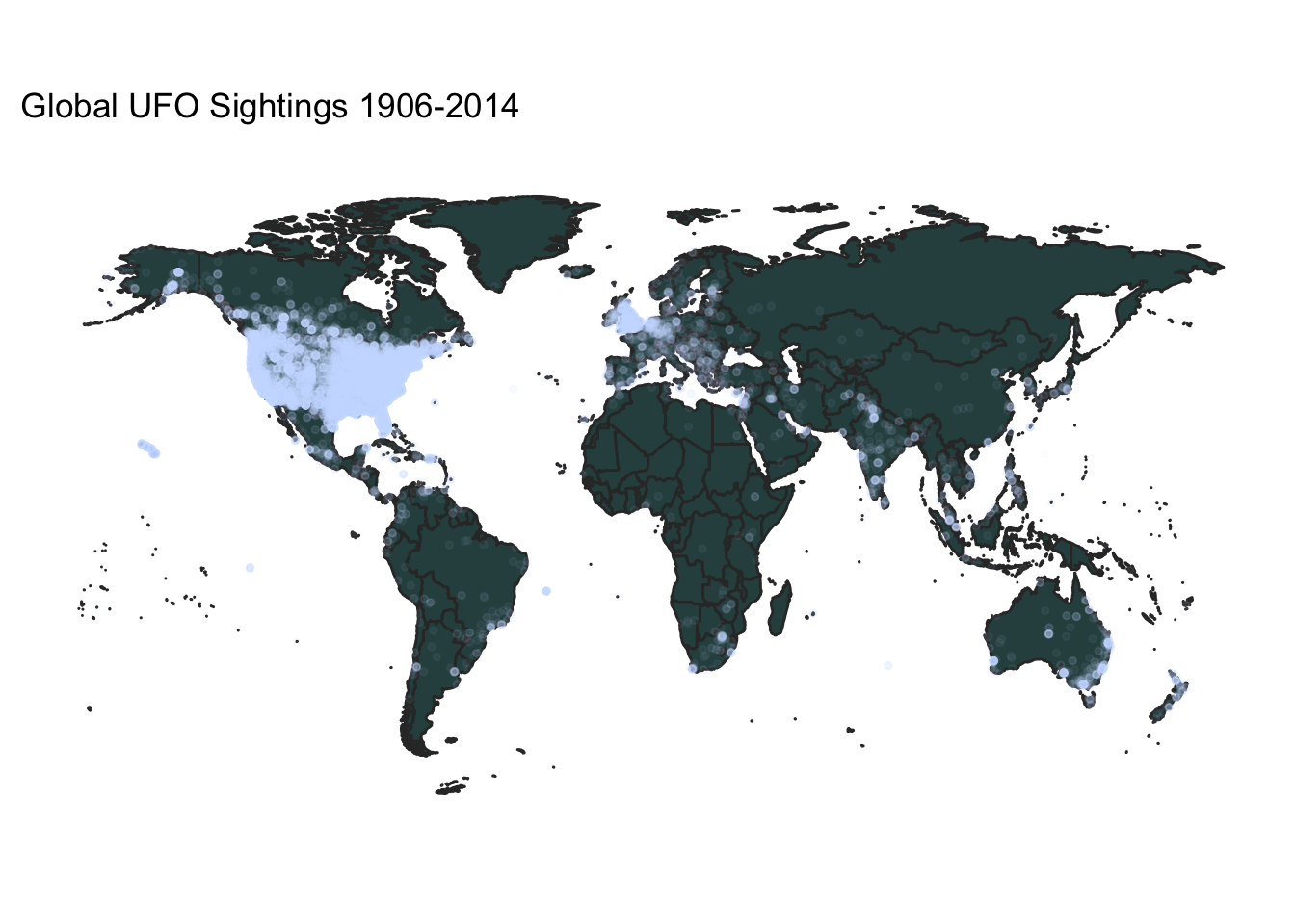
plot_ufos(n_america,ufos,
          c(-175,-45),c(10,80),
          "North American UFO Sightings 1906-2014")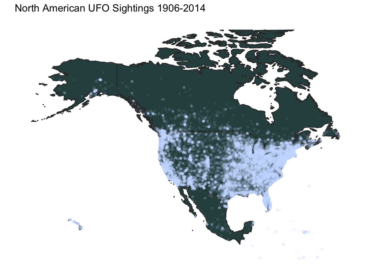
us_ufos <- ufos %>%
  filter(country == "us")

plot_ufos(states,us_ufos,
          c(-125,-65),c(25,50),
          "Lower 48 U.S. UFO Sightings 1906-2014")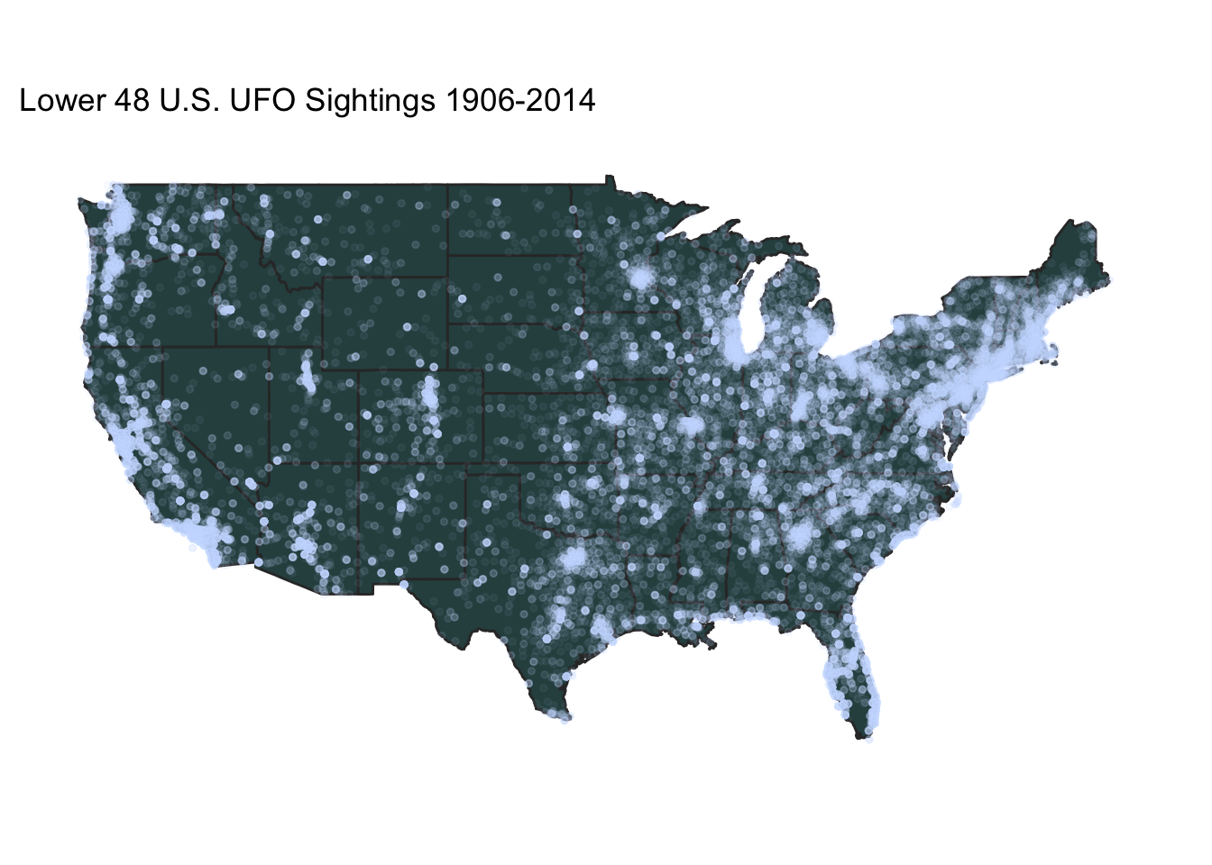
A couple observations about these maps. Obviously, given the source of this data set (an organization in Washington state), there is probably a huge American bias. Also, the organization claims to get frequent prank calls, so it is not clear how many reports are genuine. Within the U.S., the map of UFO reports looks much like a general population map, which is not surprising.
It may be interesting to next investigate the distribution of UFO sightings at each hour of the day, with the expectation that the vast majority will be at night.
ggplot(data = ufos, aes(x = hr)) +
  geom_histogram(breaks = 1:24,
                 color = "slategray1",
                 fill = "darkslategray") +
  scale_x_discrete(limits = 1:24) +
  theme(line = element_blank(),
        panel.background = element_rect(fill = "white"),
        axis.title = element_blank())+
  ggtitle("Distribution of UFO Sightings by Hour of Day 1906-2014")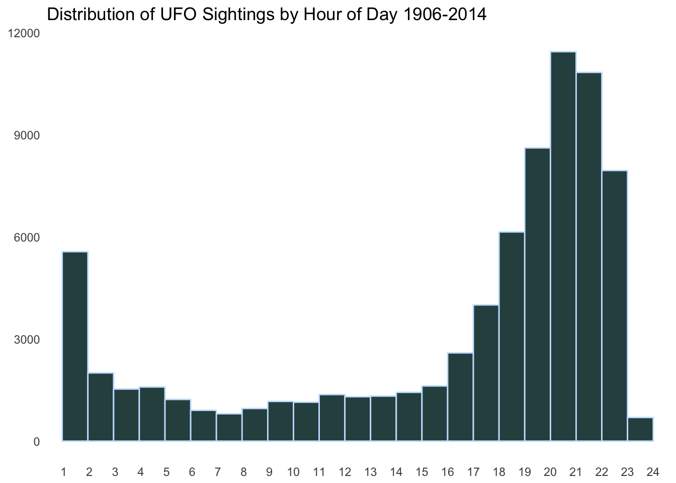
The night hours before midnight are most definitely the most popular times for UFO sightings.
ggplot(data = ufos, aes(x = date)) +
  geom_density(color = "slategray1",
               fill = "darkslategray") +
  scale_x_date() +
  theme(line = element_blank(),
        panel.background = element_rect(fill = "white"),
        axis.title = element_blank()) +
  ggtitle("Distribution of UFO Sightings by Date 1904-2014")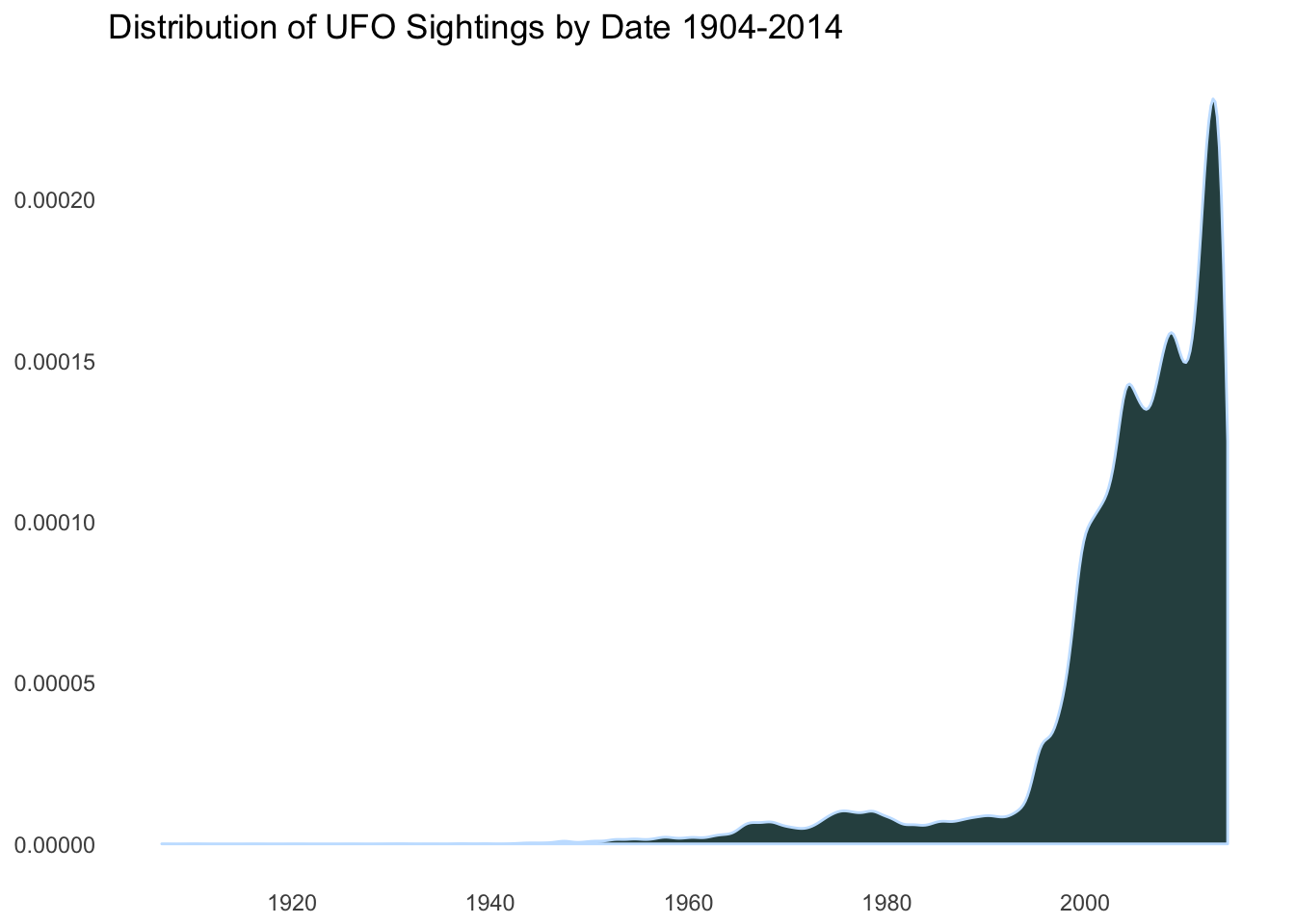
ggplot(data = ufos, aes(x = date)) +
  geom_density(color = "slategray1",
               fill = "darkslategray") +
  scale_x_date(limits = c(as.Date("2000-01-01"),
                          as.Date("2013-09-09"))) +
  theme(line = element_blank(),
        panel.background = element_rect(fill = "white"),
        axis.title = element_blank()) +
  ggtitle("Distribution of UFO Sightings by Date 2000-2014")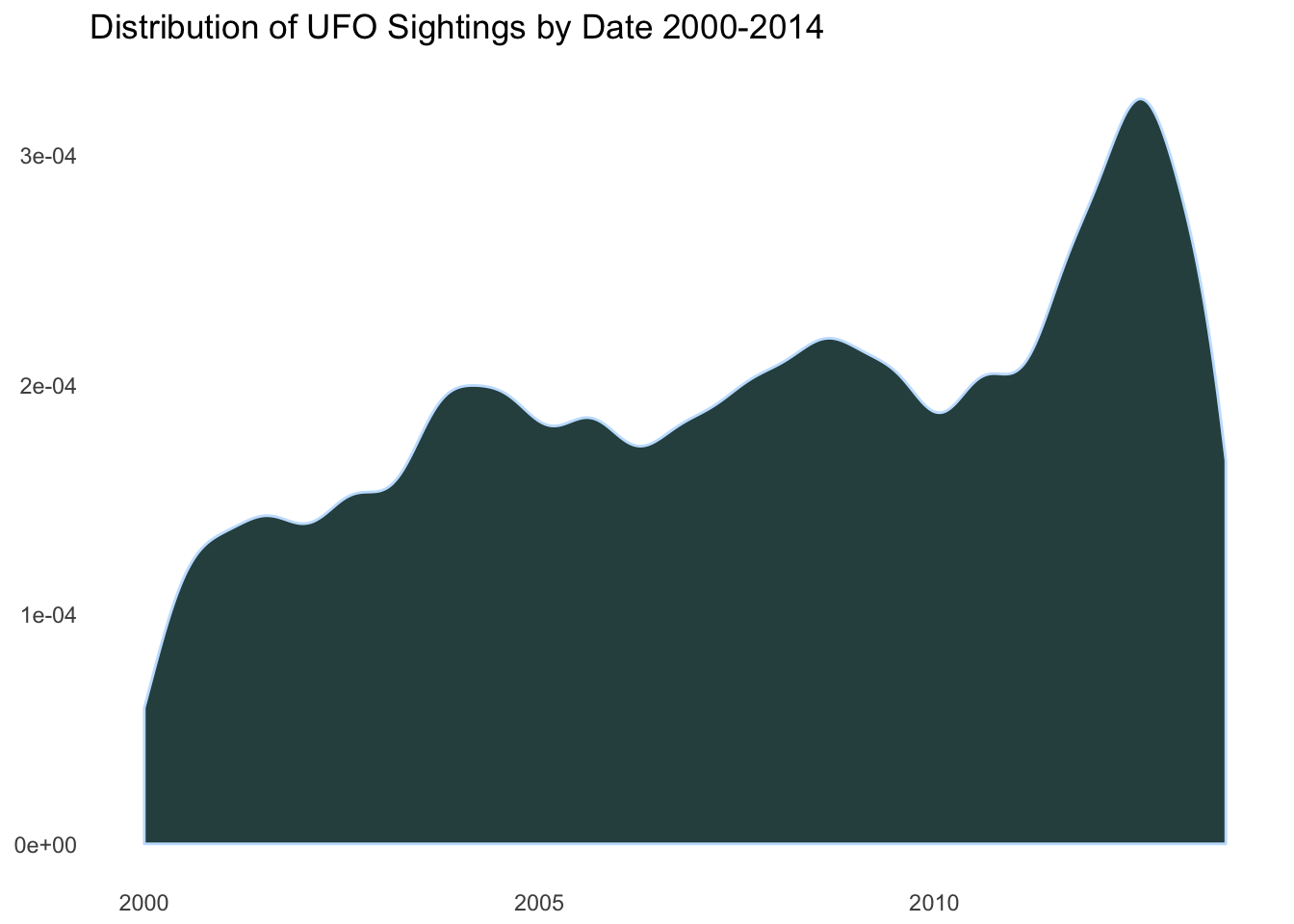
It is becoming obvious that the only real information these plots are showing is that there are more UFO sightings in more populous regions and there are more UFO sightings over time, just as there are more people over time. We will need to incorporate some new information to make any more insights into this data set.
The State Mulder-Index

We can compute a state’s Mulder-Index ™️ for a given year according to the following formula.
\[MI = 10^4 \times \frac{no. \ of \ UFO \ sightings}{state \ population}\]
To accomplish this, I will gather population estimates by state for the year 2014 from here. We now have a population estimate for each state.
pops <- read_csv("pop_est.csv")
pops
## # A tibble: 51 x 2
## state pop_2014
## <chr> <int>
## 1 al 4849377
## 2 ak 736732
## 3 az 6731484
## 4 ar 2966369
## 5 ca 38802500
## 6 co 5355866
## 7 ct 3596677
## 8 de 935614
## 9 dc 658893
## 10 fl 19893297
## # ... with 41 more rowsThe next task will be joining ufos with this new pops. An inner join will do the job.
ufos_pop <- inner_join(us_ufos,pops)Now we can compute a Mulder-Index ™️ for each state. We’ll choose the year 2012 to focus on.
ufos_pop %<>%
  filter(format(date,"%Y") == 2012) %>%
  group_by(state) %>%
  mutate(n = n(),
         mi = (n()/pop_2014)*10000) %>%
  arrange(n)
Let’s see how each state scored on the Mulder-Index ™️.
library(viridis)
ggplot() +
  geom_polygon(data = ufos_pop_mi, aes(x=long, y = lat, fill = mi,group = group)) +
  scale_fill_viridis() +
  theme(line = element_blank(),
        panel.background = element_rect(fill = "white"),
        axis.title = element_blank(),
        axis.text = element_blank()) +
  ggtitle("Mulder Index In Each State for 2012") +
  labs(subtitle = "Number of UFO Sightings per 10000 people")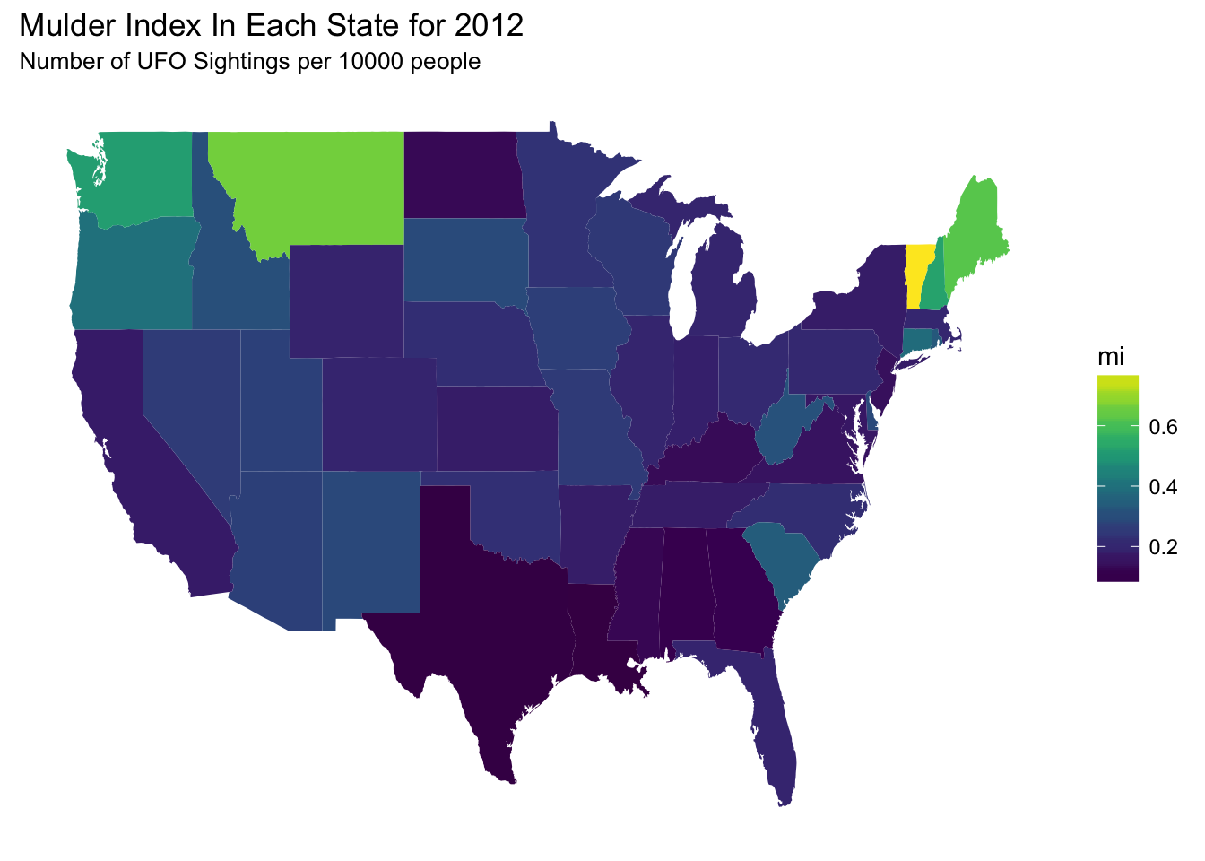
Text Analysis of Comments
Perhaps the most interesting feature of this data set are the comments included for each observation. These comments are small historical artifacts in an of themselves and they really serve to personalize each of these observations. I will first construct some simple frequency plots to get an idea for what kinds of themes are present throughout these comments.
Frequency Text Analysis
I will use the tidy text mining framework described in Text Mining with R by Julia Silge and David Robinson and implemented in the tidytext package.
library(tidytext)The comment data are already in a relatively friendly form to begin with. All we need to do is unnest each comment so that each token is a word, not a full comment, and filter our words that don’t carry much information (contained in tidytext::stop_words).
ufo_words <- ufos %>%
  select(comments) %>%
  unnest_tokens(word,comments) %>%
  anti_join(stop_words) %>%
  count(word,sort = TRUE) %>%
  filter(word != "44") # from a pervasive reserve character
I will plot the most frequent words appearing in this new ufo_words data frame, with a threshold of at least \(n = 5000\).
ufo_words %>%
  filter(n >= 5000) %>%
  ggplot(aes(x = reorder(word,-n), y = n)) +
  geom_col(color = "slategray1",
           fill = "darkslategray") +
  theme(line = element_blank(),
        panel.background = element_rect(fill = "white"),
        axis.title = element_blank()) +
  ggtitle("Most Frequent UFO Descriptors")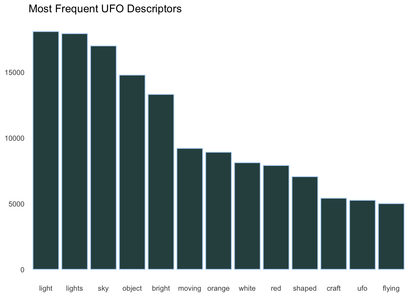
Seems like a reasonable list of words for UFO sightings! One could make the argument that “light” and “lights” should be combined but the difference may have something to say about the type of UFO spotted (i.e. whether it was a simple one light craft or a more complex multi-lighted vessel).
us_ufo_words <- ufos %>%
  filter(country == "us") %>%
  group_by(state) %>%
  select(comments) %>%
  unnest_tokens(word,comments) %>%
  anti_join(stop_words) %>%
  count(word,sort = TRUE) %>%
  filter(word != "44") %>%
  top_n(n = 4,wt = n) %>%
  arrange(state,desc(n)) %>%
  mutate(State = toupper(state))
We can check to see if there are any noticeable differences between the distribution of words over all and the distribution of words within each state in the U.S.
ggplot(us_ufo_words, aes(x = reorder(word,-n), y = n)) +
  geom_col(color = "slategray1",
           fill = "darkslategray") +
  coord_flip() +
  facet_wrap(~ State, scales = "free") +
  xlab("Word") +
  ggtitle("Top 4 UFO Comment Words in Each State") +
  theme(axis.text = element_text(size=5),
        line = element_blank(),
        panel.background = element_rect(fill = "white"),
        strip.background = element_rect(fill="darkslategray"),
strip.text = element_text(color = "slategray1")) 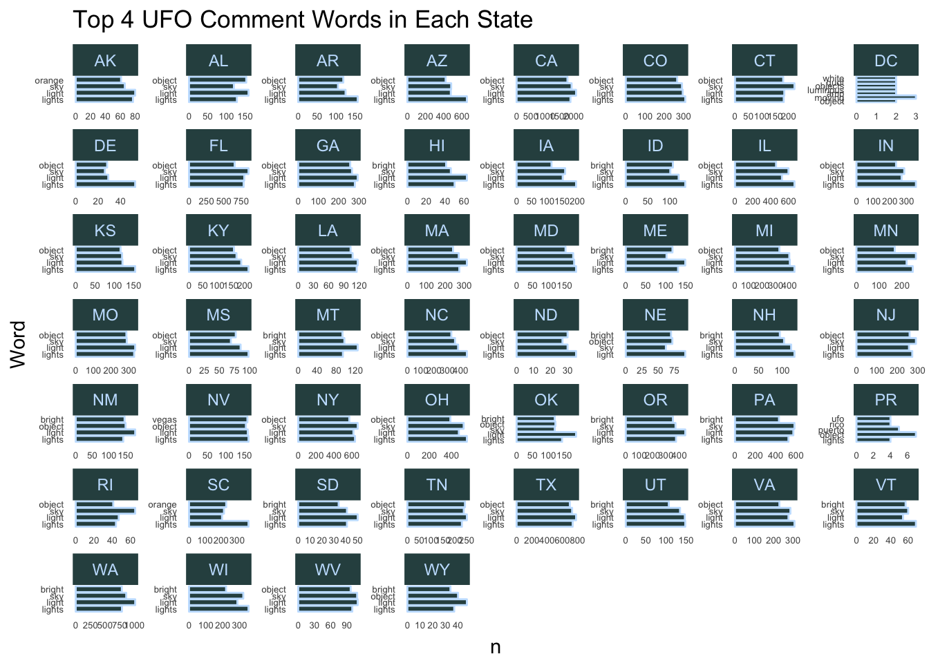
Looks like most states follow the overall trend. Note that some states have more than four in their top four because of ties.
Conclusion
Overall, this was an interesting data set with some obvious shortcomings. As is often the case, I am left with more questions than answers at this point. One thing I wonder about is to what degree the U.S. bias in this data set is attributable to any possible cultural predispositions to look for UFOs and to what degree the bias is just a function of the data coming from a U.S. source. I would also like to get more information from the comments in this data set. It might be interesting to do some kind of sentiment analysis on the comments, but I fear it may be overwhelmed by those top four or five words that pervade the comments. As for the question of whether or not any of these reports are legitimate, we may never know. But as always, the truth is out there!