Bayesian Normal Model

Inference for unknown mean and known variance

For a sampling model $Y|\mu ,{\sigma }^2\stackrel{iid}{\sim }N(\mu ,{\sigma }^2)$ we wish to make inference on $\mu$ assuming ${\sigma }^2$ is known. The first step will be to derive an expression for $\pi (\mu |Y=y,{\sigma }^2)$ which is proportional to $\pi \left(\mu |{\sigma }^2\right)\pi (y|\mu ,{\sigma }^2)$. To following prior structure will be adopted:

$$Y|\mu ,{\sigma }^2\sim N(\mu ,{\sigma }^2)$$

$$\mu \sim N({\mu }_0,{\sigma }_0^2)$$

Now we can derive an expression for $\pi (\mu |Y=y,{\sigma }^2)\propto \pi \left(\mu |{\sigma }^2\right)\pi (y|\mu ,{\sigma }^2)$.

$$\pi \left(\mu |{\sigma }^2\right)\pi (y|\mu ,{\sigma }^2)\propto e^{-\frac{1}{2{\sigma }_0^2}(\mu -{\mu }_o{)}^2}{e}^{-\frac{1}{2{\sigma }^2}(y-\mu {)}^2}$$

$$=e^{\frac{1}{2}\left(\frac{1}{{\sigma }_0^2}\right({\mu }^2-2\mu {\mu }_0+{\mu }_0^2)+\frac{1}{{\sigma }^2}(y^2-2\mu y+{\mu }^2\left)\right)}$$

Now let’s just work with the $\frac{1}{{\sigma }_0^2}({\mu }^2-2\mu {\mu }_0+{\mu }_0^2)+\frac{1}{{\sigma }^2}(y^2-2\mu y+{\mu }^2)$ by itself.

$$\frac{1}{{\sigma }_0^2}({\mu }^2-2\mu {\mu }_0+{\mu }_0^2)+\frac{1}{{\sigma }^2}(y^2-2\mu y+{\mu }^2)=\frac{{\mu }^2}{{\sigma }_0^2}-\frac{2\mu {\mu }_0}{{\sigma }_0^2}+\frac{{\mu }_0^2}{{\sigma }_0^2}+\frac{y^2}{{\sigma }^2}-\frac{2\mu y}{{\sigma }^2}+\frac{{\mu }^2}{{\sigma }^2}$$

$$={\mu }^2(\frac{1}{{\sigma }_0^2}+\frac{1}{{\sigma }^2})-2\mu (\frac{{\mu }_0}{{\sigma }_0^2}+\frac{y}{{\sigma }^2})+\frac{{\mu }_0^2}{{\sigma }_0^2}+\frac{y^2}{{\sigma }^2}$$

To get this final expression into a quadratic form we can let $a=\frac{1}{{\sigma }_0^2}+\frac{1}{{\sigma }^2}$, $b=\frac{{\mu }_0}{{\sigma }_0^2}+\frac{y}{{\sigma }^2}$, and $c=\frac{{\mu }_0^2}{{\sigma }_0^2}+\frac{y^2}{{\sigma }^2}$. In proportionality the $c$ term will drop from the exponent. Now we have

$$\pi (\mu |{\sigma }^2,y)\propto e^{-\frac{1}{2}(a{\mu }^2-2b\mu )}=e^{-\frac{1}{2}a({\mu }^2-2b\mu /a+b^2/a^2)+b^2/2a}$$

$$=e^{-\frac{1}{2}a(\mu -b/a{)}^2}=e^{-\frac{1}{2}(\frac{\mu -b/a}{1/\sqrt{a}}{)}^2}$$

Which is recognizable as the kernel of a $N(b/a,1/a)=N({\mu }_n=\frac{\frac{{\mu }_0}{{\sigma }_0^2}+\frac{y}{{\sigma }^2}}{\frac{1}{{\sigma }_0^2}+\frac{1}{{\sigma }^2}},{\sigma }_n^2=\frac{1}{\frac{1}{{\sigma }_0^2}+\frac{1}{{\sigma }^2}})$.

Inference for unknown mean and unknown variance

It is more reasonable to expect that in an actual data analysis if we are trying to estimate the mean of a normal population then we likely need to estimate the variance as well. The following parameterization is used by Hoff in A First Course in Bayesian Statistical Methods.

$$1/{\sigma }^2\sim gamma(shape=\frac{{\nu }_0}{2},rate=\frac{{\nu }_0{\sigma }_0^2}{2})$$

$$\mu |{\sigma }^2\sim N({\mu }_0,\frac{{\sigma }^2}{{\kappa }_0})$$

$$Y_1,...,Y_n|\mu ,{\sigma }^2\stackrel{iid}{\sim }N(\mu ,{\sigma }^2)$$

The posterior joint distribution of $\mu ,{\sigma }^2$ after observing the data $Y_1,...,Y_n$ is given by the following product.

$$\pi (\mu ,{\sigma }^2|y_1,...,y_n)=\pi (\mu |{\sigma }^2,y_1,...,y_n)\pi ({\sigma }^2|y_1,...,y_n)$$

This first term $\pi (\mu |{\sigma }^2,y_1,...,y_n)$ is the conditional posterior distribution of $\mu$. Since it is conditional on ${\sigma }^2$ (i.e. ${\sigma }^2$ is “known”) it can be derived with a calculation identical to the one given in the previous section. Generalizing to a sample of size $n$ instead of size 1 and substituting ${\sigma }^2/{\kappa }_n$ for ${\sigma }_0^2$ we get that

$$\mu |y_1,...,y_n,{\sigma }^2\sim N({\mu }_n=\frac{{\kappa }_0{\mu }_0+n\overline{y}}{{\kappa }_n},\frac{{\sigma }^2}{{\kappa }_n})$$

where ${\kappa }_n={\kappa }_0+n$. Hoff’s parameterization lends itself to a nice interpretation of ${\mu }_0$ and the mean of ${\kappa }_0$ prior observations and ${\mu }_n$ as the mean of ${\kappa }_0$ prior observations and $n$ new observations all together. Also, the variance of $\mu |y_1,...,y_n,{\sigma }^2$ is ${\sigma }^2/{\kappa }_n$.

Now to get the posterior distribution of ${\sigma }^2$ after observing $y_1,...,y_n$ we need to integrate over all possible values of $\mu$ according to

$$\pi ({\sigma }^2|y_1,...,y_n)\propto \pi \left({\sigma }^2\right)\pi (y_1,...,y_n|{\sigma }^2)$$

$$=\pi \left({\sigma }^2\right){\int }_{\mu }\pi (y_1,...,y_n|\mu ,{\sigma }^2)\pi \left(\mu |{\sigma }^2\right)d\mu$$

$$=\pi \left({\sigma }^2\right){\int }_{\mu }\left(\frac{1}{2\pi {\sigma }^2}{)}^{-n/2}{e}^{-\frac{\sum (y_i-\mu {)}^2}{2{\sigma }^2}}\right(\frac{1}{2\pi {\sigma }^2/{\kappa }_0}{)}^{-1/2}{e}^{-\frac{(\mu -{\mu }_0{)}^2}{2{\sigma }^2/{\kappa }_0}}d\mu$$

Eventually, we get that ${\sigma }^2|y_1,...,y_n\sim IG({\nu }_n/2,{\nu }_n{\sigma }_n^2/2)$ or alternatively $1/{\sigma }^2|y_1,...,y_n\sim Gamma({\nu }_n/2,{\nu }_n{\sigma }_n^2/2)$, where

$${\nu }_n={\nu }_0+n$$

$${\sigma }_n^2=\frac{1}{{\nu }_n}[{\nu }_0{\sigma }_0^2+(n-1)s^2+\frac{{\kappa }_{0}n}{{\kappa }_n}(\overline{y}-{\mu }_0{)}^2]$$

We get another nice interpretation here of ${\nu }_0$ as the prior sample size with corresponding sample variance ${\sigma }_0^2$. Also $s^2$ is the sample variance and $(n-1)s^2$ is the sample sum of squares.

normR

# devtools::install_github("carter-allen/normR")
library(normR)

Monte Carlo Sampling

Example from Hoff pg. 76.

# parameters for the normal prior
mu_0 <- 1.9
kappa_0 <- 1

# parameters for the gamma prior
sigsq_0 <- 0.010
nu_0 <- 1

# some data 
ys <- c(1.64,1.70,1.72,1.74,1.82,1.82,1.82,1.90,2.08)
n <- length(ys)
y_bar <- mean(ys)
ssq <- var(ys)

# posterior parameters
kappa_n <- kappa_0 + n
nu_n <- nu_0 + n
mu_n <- mu_n(kappa_0,mu_0,n,y_bar)
sigsq_n <- sigsq_n(nu_0,sigsq_0,n,ssq,kappa_0,y_bar,mu_0)

mu_n

## [1] 1.814

sigsq_n

## [1] 0.015324

# posterior variance draws
sigsq_posterior_draw <- draw_sigsq_posterior(10000,nu_n,sigsq_n)
# posterior mean draws
mu_posterior_draw <- draw_mu_posterior(mu_n,sigsq_posterior_draw,kappa_n)

quantile(mu_posterior_draw,c(0.025,0.975))

##     2.5%    97.5% 
## 1.727323 1.899154

# plot posterior draws
normR::plot_monte_sim(sigsq_posterior_draw,mu_posterior_draw)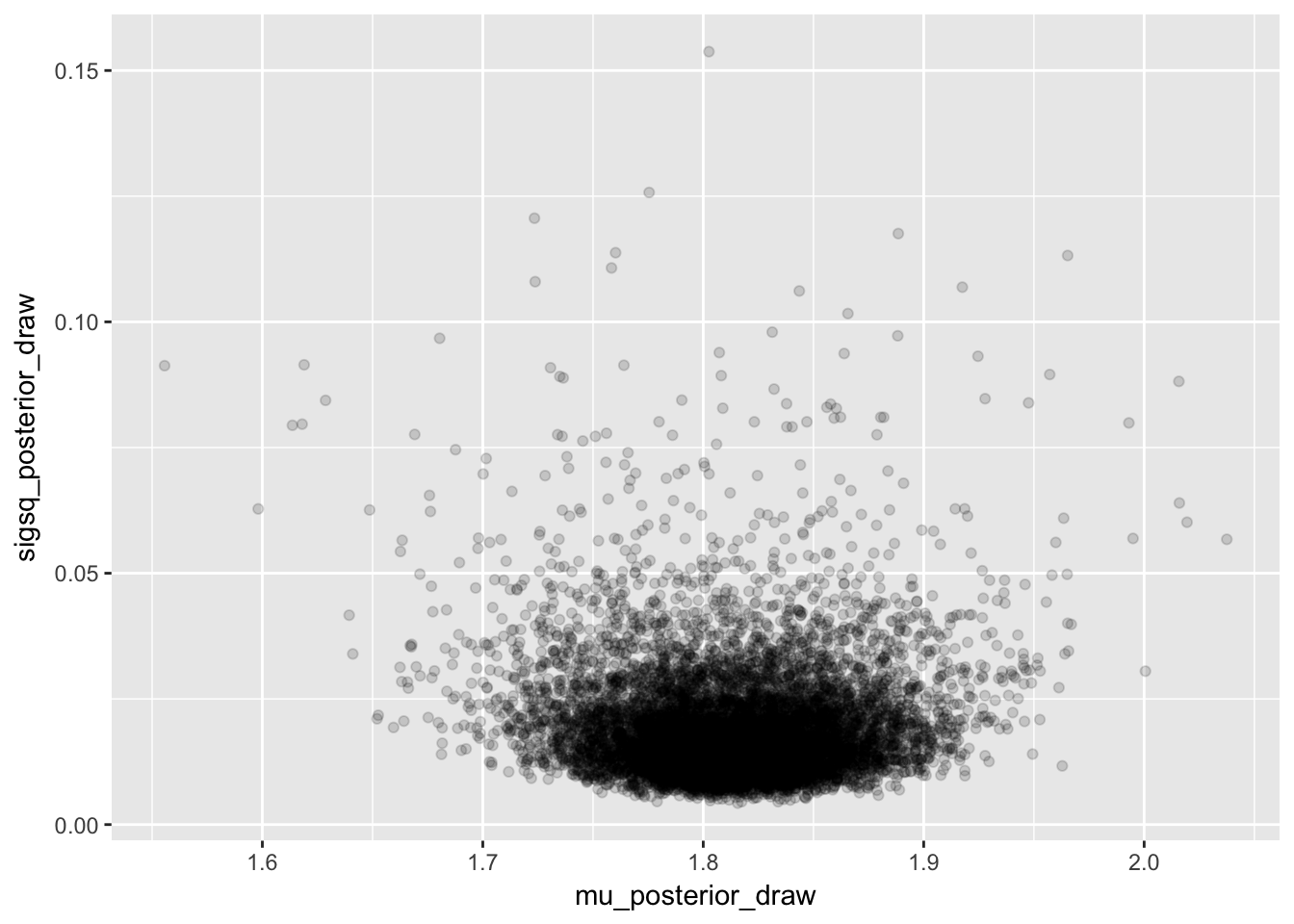

# plot posterior density estimate for sigma
normR::plot_posterior_density_estimate(sigsq_posterior_draw,
                                       plot_title = "Posterior density estimate of sigma")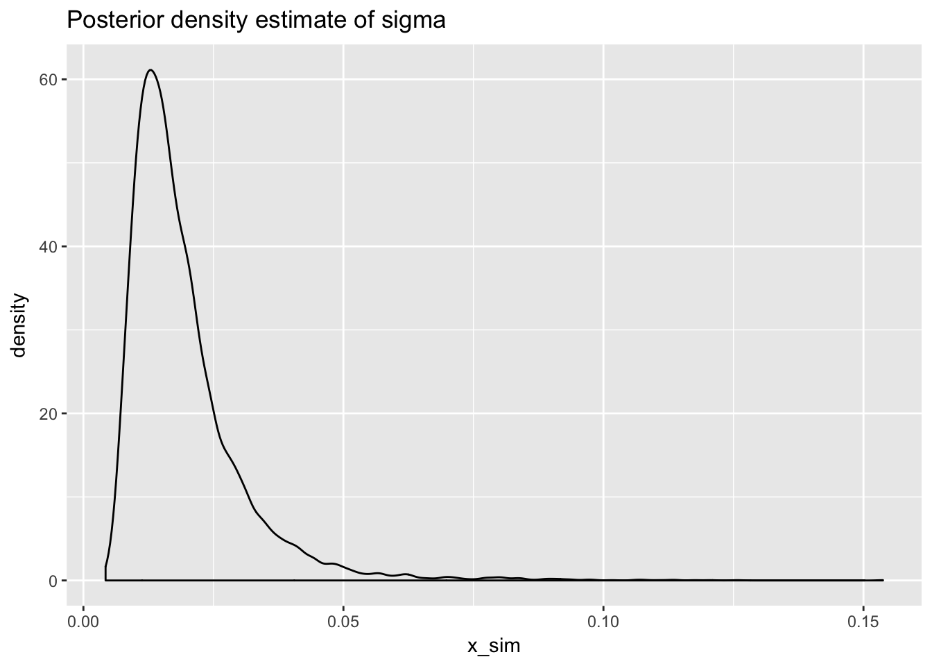

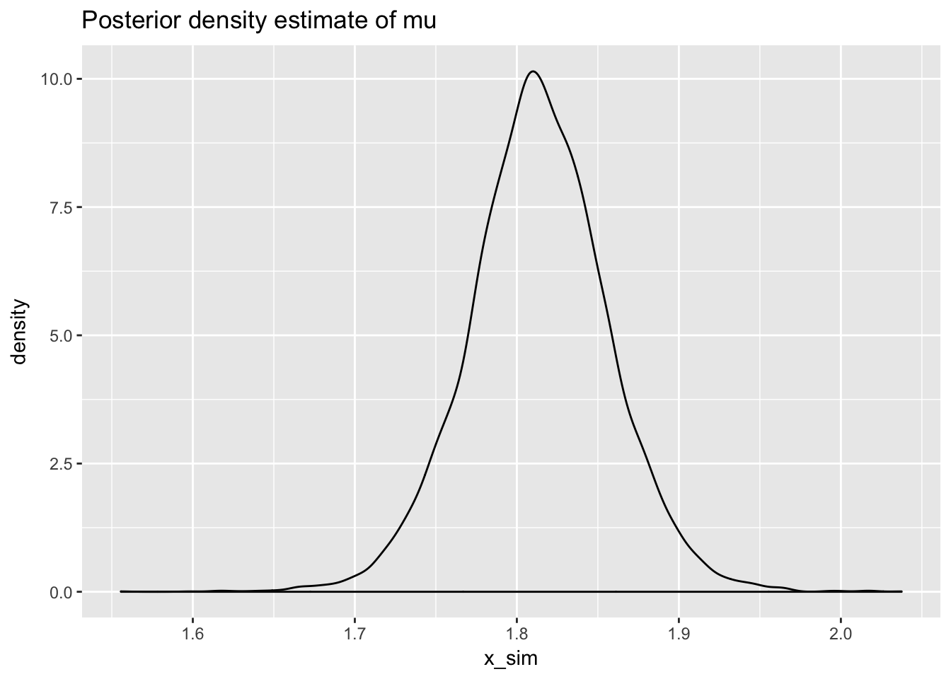
# posterior density estimate of mu
normR::plot_posterior_density_estimate(mu_posterior_draw,
                                       plot_title = "Posterior density estimate of mu")

Shiny App

https://carter-allen.shinyapps.io/NormalModel/