Bayesian Inference with Count Data
If we model the count of events \(X\) over a certain interval as a Poisson random variable with rate \(\lambda\), then \(X|\lambda \sim Poisson(\lambda)\). This can be thought of as a prior model for \(X\), where \(\lambda\) is itself a random variable. We can adopt a \(Gamma(\alpha,\beta)\) prior for \(\lambda\) to allow for conjugacy of the prior and posterior.
To derive the posterior and predictive distributions, we first need to find the joint distribution of \(X\) and \(\lambda\), \(f(x,\lambda)\). Using the shape-scale parameterization of the Gamma, the joint distribution is
\[f(x,\lambda)=f(x|\lambda)f(\lambda)=[\frac{\lambda^x e^{-\lambda}}{x!}][\frac{1}{\beta^\alpha \Gamma(\alpha)}\lambda^{\alpha-1}e^{-\lambda/\beta}]\]
The prior predictive distribution of \(X\) (the marginal of \(X\)) is given by
\[f(x) = \int_\lambda f(x,\lambda)d\lambda = \frac{1}{\beta^\alpha \Gamma(\alpha)x!}\int_0^\infty \lambda^{\alpha-1+x} e^{-\lambda(1+\frac{1}{1+\beta})}\]
Inside this last integral is the kernel of another random variable, a \(Gamma(\alpha+x,\frac{\beta}{\beta+1})\), which integrates over its whole support to \(\Gamma(\alpha+x)(\frac{\beta}{\beta+1})^{\alpha+x}\).
\[\Rightarrow f(x) = \frac{\Gamma(\alpha+x)(\frac{\beta}{\beta+1})^{\alpha+x}}{\beta^\alpha \Gamma(\alpha) \Gamma(x+1)}=\frac{(\alpha-1+x)!}{(\alpha-1)!(x)!} \frac{\beta^{\alpha+x}(\frac{1}{\beta+1})^{\alpha+x}}{\beta^{\alpha}}\]
\[= {{\alpha+x-1}\choose{x}} (\frac{1}{\beta+1})^{\alpha}(1-\frac{1}{1+\beta})^{x}\]
This final expression for \(f(x)\) is the pmf of a Negative Binomial random variable with parameters \(r=\alpha\) and \(p=\frac{1}{1+\beta}\) that models the number of failures before the \(r^{th}\) success.
If we were to have used the shape-rate parameterization of the Gamma, this prior predictive would end up being a Negative Binomial with \(r=\alpha\) and \(p=\frac{\beta}{1+\beta}\).
The posterior distribution for \(\lambda\) after observing \(X=x\) using the shape-scale parameterization is
\[f(\lambda|X=x) = \frac{f(\lambda,x)}{f(x)}=\frac{\frac{\lambda^{\alpha-1+x}e^{-\lambda(1+1/\beta)}}{\beta^\alpha \Gamma(\alpha) x!}}{\frac{\Gamma(\alpha+x)(\frac{\beta}{\beta+1})^{\alpha+x}}{\beta^\alpha \Gamma(\alpha) x!}} = \frac{1}{\Gamma(\alpha+x)(\frac{\beta}{\beta+1})^{\alpha+x}}\lambda^{\alpha-1+x}e^{-\lambda(1+1/\beta)}\]
which is the pdf of a \(Gamma(\alpha+x,\frac{\beta}{1+\beta})\) random variable.
Under the shape-rate parameterization this posterior would be a \(Gamma(\alpha+x,\beta+1)\).
The final distribution of interest is that of the posterior predictive of a new observation denoted \(X^*\) after already observing that \(X=x\). It is a bit simpler to see the derivation using the shape-rate parameterization of the Gamma distribution.
\[f(x^*|X=x) = \int_\lambda f(x^*|\lambda,x)f(\lambda|x)d\lambda=\int_0^\infty f(x^*|\lambda)f(\lambda|x)d\lambda\]
\[=\int_0^\infty \frac{e^{-\lambda}\lambda^{x^*}}{x!} \frac{(\beta+1)^{\alpha+x}}{\Gamma(\alpha+x)} \lambda^{\alpha+x-1}e^{-\lambda(\beta+1)} d\lambda\]
After integrating the kernel of a \(Gamma(\alpha+x+x^*,\beta+2)\) density contained in the above expression, the posterior predictive simplifies to the pmf of a Negative Binomial with \(r = \alpha+x\) and \(p = \frac{\beta + 1}{\beta+2}\).
Random Sample of Size n
The above derivations deal with observing a single value of a random variable \(X=x\). These results can generalized to observing values of a random sample of \(n\) identically distributed \(Poisson(\lambda)\) random variables \(X_1 = x_1,X_2 = x_2,...,X_n=x_n\).
The posterior distribution of \(\lambda\) after observing the random sample \(X_1 = x_1,X_2 = x_2,...,X_n=x_n\) is a \(Gamma(\sum_{i=1}^{n} x_i + \alpha,n+\beta)\), using the shape-rate Gamma parameterization.
The posterior predictive distribution of a new variable \(X^*\) after observing the random sample \(X_1 = x_1,X_2 = x_2,...,X_n=x_n\) is a Negative Binomial with \(r =\alpha+\sum x_i,p=\frac{\beta+n}{\beta+n+1}\), using the shape-rate Gamma parameterization.
Useful R Functions
Some useful functions for plotting the Gamma, Negative Binomial, and Poisson variables that arise in Gamma Poisson modeling are included in the gammaR function, installable with the following command.
devtools::install_github("carter-allen/gammaR")The functions dgam_plot(), dnb_plot(), and dpois_plot() can be used to quickly plot Gamma, Negative Binomial, and Poisson distributions, respectively.
Example
library(gammaR)Imagine the situation of modeling the number of unhappy customers that will arrive at an ice cream shop per day at the beginning of the week, and then updating this model for the rest of the week after Monday. We can adopt a \(Poisson(\lambda)\) likelihood model for the number of unhappy customers arriving per hour \(X\) on any given day. If we know that on Friday 6 unhappy customers came to the shop, we can adopt a \(Gamma(\alpha = 6, \beta = 1)\). Here alpha = 6 can be interpreted as the sum of prior counts and beta = 1 can be interpreted as the number of trials. Note that the shape-rate parameterization is being used here for the Gamma distribution. The prior distribution has the following shape.
dgam_plot(alpha,beta)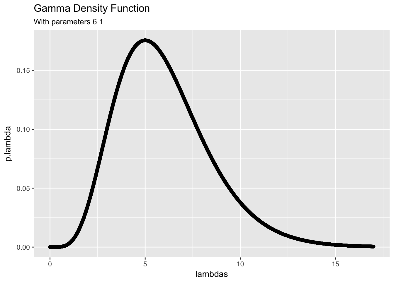
From the derivations above, we can see that the marginal distribution of \(X\), the prior predictive distribution of \(X\) before observing any new data, is a Negative Binomial distribution with \(r = \alpha\) and \(p = \frac{1}{1+\beta}\) and the following shape.
dnb_plot(alpha,beta/(1+beta))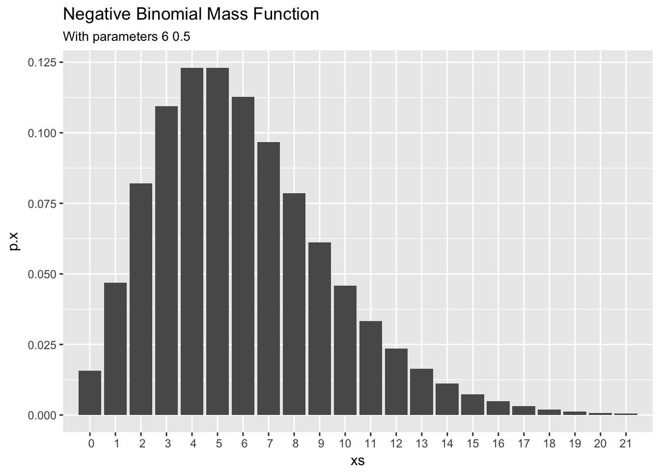
Now if at the end of the day on Monday we record that only x = 3 unhappy customers visited the shop, we can use this information to update our belief about the distribution of \(\lambda\), the average number of grumpy customers per day. The posterior distribution of \(\lambda|X=3\) is a \(Gamma(\alpha+x,\beta + n)\), where n = 1 corresponds to the single day observed. The posterior has the following shape.
dgam_plot(alpha + x, beta + n)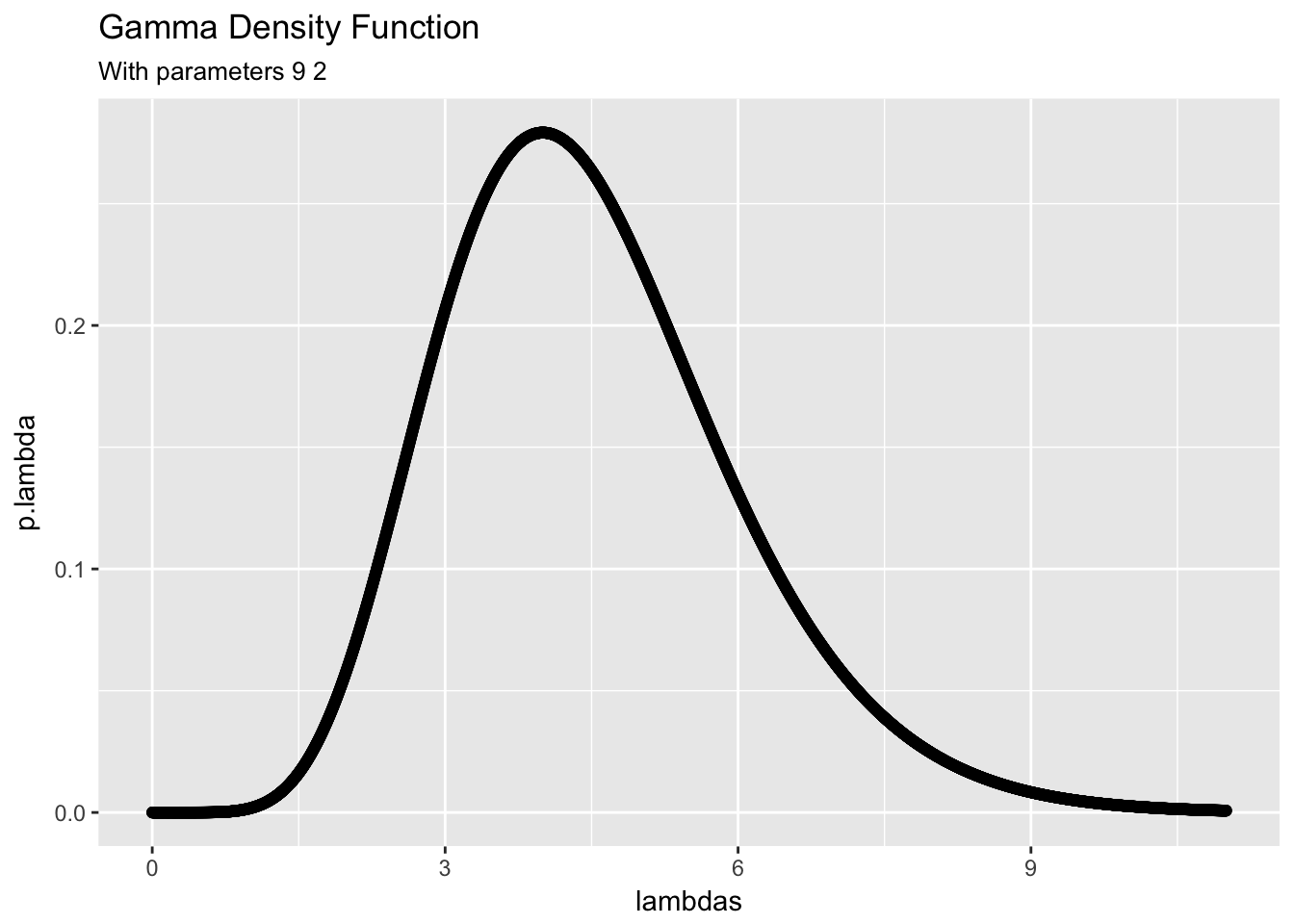
Note that the scaling of this posterior is different from the prior and the posterior has more density on lower values of \(\lambda\).
Finally, the posterior predictive distribution of the number of unhappy customers that will come to the ice cream shop tomorrow \(X^*\) is a Negative Binomial with \(r = \alpha + x\) and \(p = \frac{\beta+n}{\beta+n+1}\), which has the following shape.
dnb_plot(alpha + x,(beta+n)/(beta+n+1))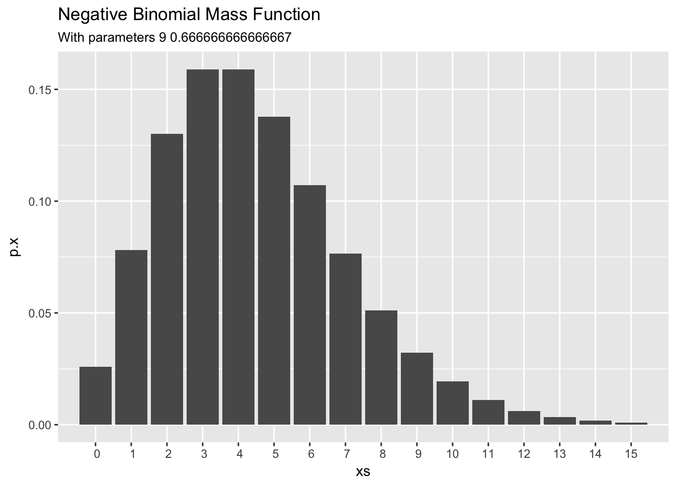
Shiny App
A online applet for tweaking these parameters and visualizing the models in this distribution can be found at https://carter-allen.shinyapps.io/GammaPoisson/.