Bayesian Inference with Binary Data
The Beta-Binomial model is a classic Bayesian framework for working with dichotomous data. If we observe a Bernoulli process over a total of \(n\) trials, where each trial has “success” probability \(\theta\), then the total number of successes in \(n\) trials \(X\) is a binomial random variable where \(X = 0,1,2,...,n\).
\[p(X=x|\theta) = {{n}\choose{x}} \theta^x (1-\theta)^{n-x}\]
The binomial random variable is known as the likelihood of this model. Now, if there is uncertainty about the parameter \(\theta\) in the binomial model, we can treat \(\theta\) as an additional random variable that follows a \(beta(\alpha,\beta)\) distribution where \(0 \le \theta \le 1\).
\[p(\theta) = \frac{\Gamma(\alpha,\beta)}{\Gamma(\alpha) \Gamma(\beta)} \theta ^{\alpha-1} (1-\theta)^{\beta-1}\]
The beta distribution is the prior for this model. Given we know \(X=x\) successes occured over \(n\) trials of the Bernoulli process with success probablility \(\theta\), we can derive the posterior distribution for \(\theta\), that is, the distribution of \(\theta\) that incorporates prior information and observed information, namely the quantity \(X=x\).
\[p(\theta|X=x) \propto \theta^x (1-\theta)^{n-x} \theta ^{\alpha-1} (1-\theta)^{\beta-1}\]
\[= \theta^{x+\alpha-1} (1-\theta)^{n-x+\beta-1}\]
This expression has the form of the kernel of another beta distribution with parameters \(\alpha^* = x + \alpha\) and \(\beta^* = n-x+\beta\)
To find the predictive distribution of \(X\), \(f_X(x)\), we first need the joint distribution of \(X\) and \(\theta\), \(f_{X,\theta}(x,\theta)\).
\[f_{X,\theta}(x,\theta) = f_{\theta}(\theta) f_{X|\theta}(x|\theta) = \frac{\Gamma(\alpha,\beta)}{\Gamma(\alpha) \Gamma(\beta)} {{n}\choose{x}} \theta^{\alpha+x-1} (1-\theta)^{\beta + n -x -1}\]
The prior predictive distribution \(f_X(x)\) = \(\int_{\theta} f_{X,\theta}(x,\theta) d\theta\).
\[\int_{\theta} \frac{\Gamma(\alpha,\beta)}{\Gamma(\alpha) \Gamma(\beta)} {{n}\choose{x}} \theta^{\alpha+x-1} (1-\theta)^{\beta + n -x -1} d\theta\] \[=\frac{\Gamma(\alpha,\beta)}{\Gamma(\alpha) \Gamma(\beta)} {{n}\choose{x}} \frac{\Gamma(\alpha + x) \Gamma(\beta+n-x)}{\Gamma(\alpha+x,\beta+n-x)}\]
\[={{n}\choose{k}} \frac{B(\alpha + x, \beta + n-x)}{B(\alpha,\beta)}\]
The above expression is the probability density function of a beta-binomial random variable with parameters \(n,\alpha,\beta\). This is the distribution of \(X\) averaged over all possible values of \(\theta\).
The last distribution of interest in this model is the posterior predictive distribution, of the predictive distribution of a new \(X\) (call it \(X^*\)) an observation \(X=x\).
\[f_{X^*|X=x}=\int_{\theta} f(x^*|\theta,x)f(\theta|x)d\theta\] Since \(X^*\) and \(X\) are conditionally independent given \(\theta\),
\[= \int_{\theta} f(x^*|\theta)f(\theta|x)d\theta\]
Following a similar derivation as that of the prior predictive, \(X^* \sim beta \ binom(n,x+\alpha,n-x+\beta)\).
Useful R Functions
The betaR package includes some useful functions for working with the beta binomial model. The package can be found at https://github.com/carter-allen/betaR, and installed using the following command.
devtools::install_github("carter-allen/betaR")Example
library(betaR)Consider the situation in which we are we are modeling a team’s number of wins over a \(n=12\) game season. The probability that the team wins any given game \(\theta\) is probably not a fixed value, with variability coming from the quality of the opposing team, home-court advantage, and countless other factors. If the team is relatively good though, we might expect their probability of winning any given game to be around \(\theta = 0.75\), but not fixed at \(\theta=0.75\).
We can represent this prior belief by a beta distribtibution for \(\theta\) with parameters \(\alpha = 9\) and \(\beta = 3\). These parameters can be thought of as the number of prior wins and prior losses respectively, and would be a reasonable assumption if the team went 9-3 last season. The prior distribution of \(\theta\) is shown below.
dbeta_plot(alpha = 9, beta = 3)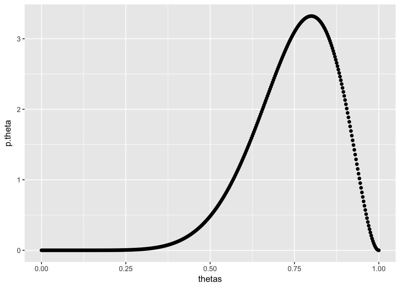
Now if we wanted to make a prediction about how the team will do this season, we can form a prior predictive distribution of \(X\), that is, the number of games we expect the team to win this season, given their 9-3 record last season. If we model each game by a \(binomial(n = 12,p = \theta)\) distribution and keep our \(beta(\alpha = 9,\beta = 3)\) prior for \(\theta\), the prior predictive distribution of \(X\) is a \(beta \ binomial(n = 12,\alpha = 9,\beta = 3)\). The prior predictive distribution of \(X\) is shown below. Note the similarity in shape to the prior.
dbb_plot(n = 12, alpha = 9, beta = 3)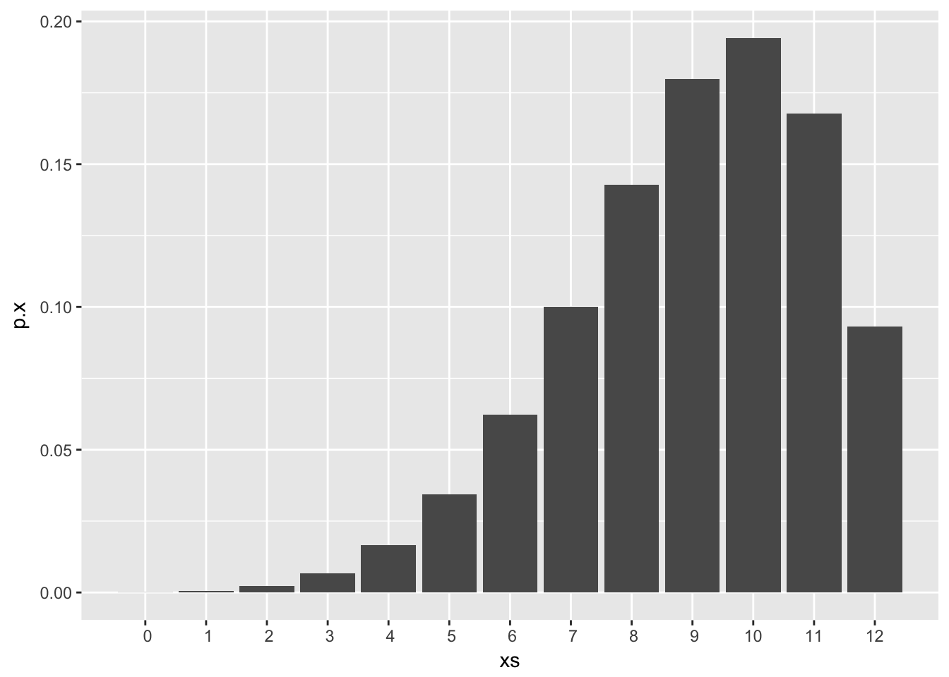
Let’s say that the season we are predicting ends up being much less successful than we expected, with the team going 4-8 over 12 games. Given this information, we can update our knowledge about \(\theta\), the probability that this team wins any given game. \(\theta|X=x \sim beta(x+\alpha,n-x+\beta) = beta(4+9,12-4+3)\), which has the following distribution.
dbeta_plot(alpha = 4+9,beta = 12-4+3)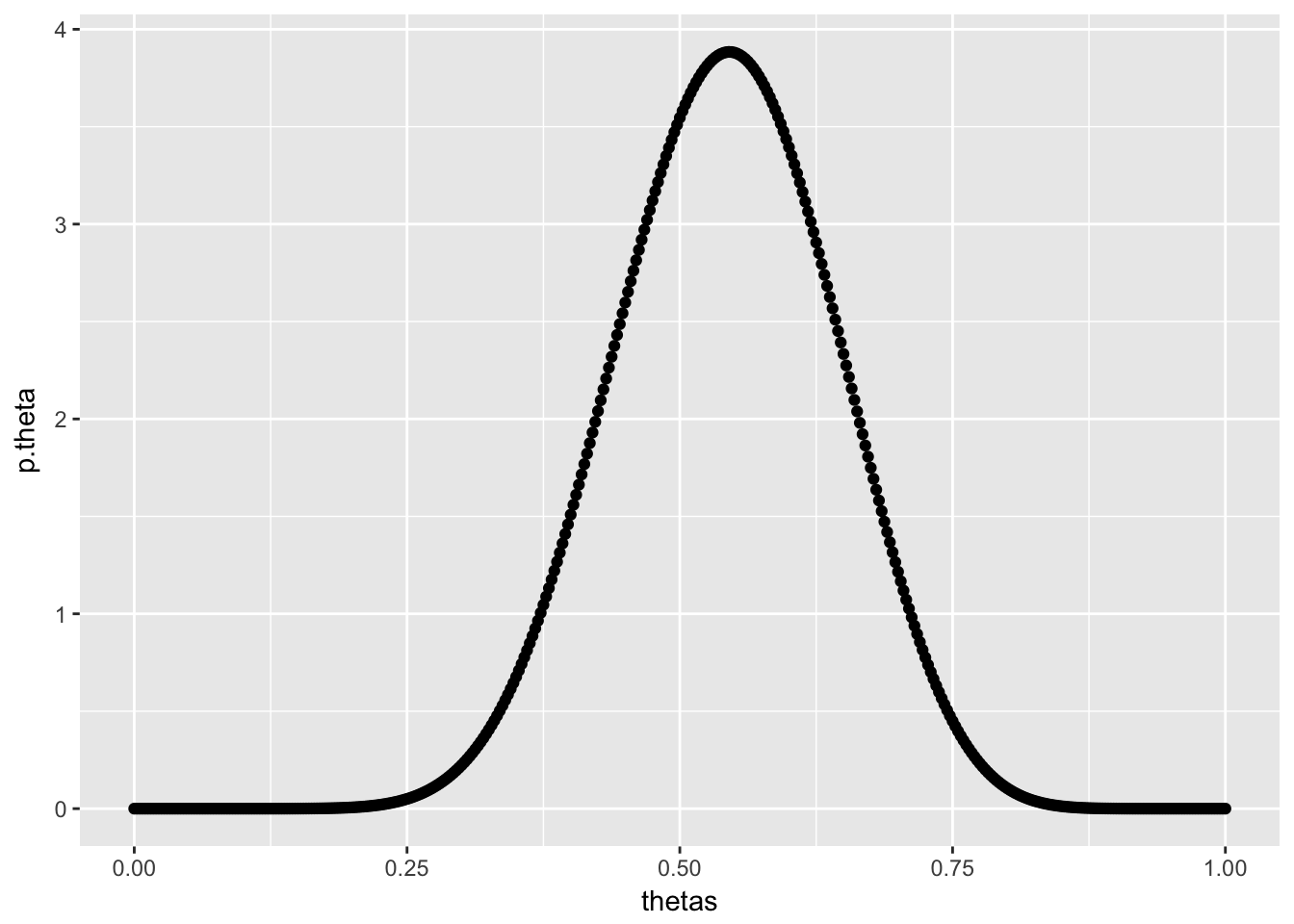
Our belief about the probability this team wins any given game has become a bit less optimistic given their dissapointing last season.
Finally, lets take into account all of this information from the past two seasons to get a posterior predictive distribution of a new 12 game season. From earlier, \(X^* \sim beta \ binom(n,x+\alpha,n-x+\beta) = beta \ binom(12,4+9,12-4+3)\)
dbb_plot(n = 12, alpha = 4+9, beta = 12-4+3)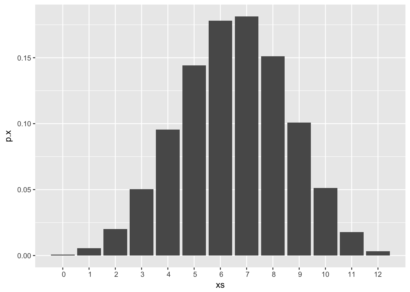
Shiny App
The reactive app for visualizing the distributions discussed here under different parameter sets can be found at https://carter-allen.shinyapps.io/BetaBinomial/.