Approved by:
Primary Advisor: Dr. Edsel Peña; Professor, Dept. of Statistics
Second Reader: Dr. John Grego; Professor & Chair, Dept. of Statistics
Submitted in partial fulfillment of the requirments for
graduation with Honors from the South Carolina Honors College.

Abstract
This project addresses the need for predictive modeling tools to forecast expected concentrations of fecal bacteria in recreational waters in the Charleston, SC area. Data was provided by Charleston Waterkeeper, a water quality monitoring organization that has been measuring Enterococcus faecalis concentrations at 15 recreational sites since 2013. The data contain a non-negligible number of censored and missing observations, so three distinct imputation methods were developed and compared in terms of their effect on final predictive model characteristics. The best performing method relied on drawing samples from a truncated normal distribution to replace censored values, and using a partial model built from all non-missing observations to impute missing values. Finally, a predictive model of Enterococcus in terms of precipitation in the past 72 hours, tidal stage, and sample site was developed. Results from this project may be used for forecasting Enterococcus concentrations in practice, as well as for informing the imputation phases of future studies.
Personal Motivation
The origins of this research date back to the beginning of my involvement with Charleston Waterkeeper, a non-profit water quality monitoring organization based in Charleston, SC. I first discovered Charleston Waterkeeper during the Spring semester of my sophomore year at the University of South Carolina after reading The Riverkeepers by Robert F. Kennedy Jr. and John Cronin, a book that details the formation of the now international Waterkeeper Alliance [1]. Charleston Waterkeeper, a member of the Waterkeeper Alliance, relies on volunteer service to sustain their water quality monitoring program, a volunteer program through which I first became involved with the organization.
The following fall semester, I began taking upper level classes for my major in statistics at the University of South Carolina. The material covered in these introductory courses was foundational to completing this project, and highly applicable to the work I was doing the previous summer with Charleston Waterkeeper. Over the course of that year, I became familiar with statistical methods and tools that struck me as being highly applicable to Charleston Waterkeeper’s water quality monitoring program. With a lifelong interest in environmental sciences and a major in statistics, I decided that building a predictive water quality model would be a perfect application of my major to a meaningful problem.
To me, this thesis embodies the ability for research in statistics to occupy the intersection of natural science, mathematics, and computer science, among other areas. As a truly interdisciplinary subject, research in statistics often requires proficiency in programming languages to run simulations and analyses, knowledge of mathematics to prove underlying principles, and a familiarity with the project’s area of application to guide and contextualize the analysis. Most importantly, a grasp of fundamental statistical theorems and methods is necessary to perform the modeling of natural phenomena. These are all skills that I was introduced to through coursework at USC. I am grateful to my professors and mentors who have challenged me to learn this material both in and out of the classroom.
A Note on Reproducibility
This thesis was written entirely using R Markdown, a document format provided by R Studio for creating technical documents in R [2]. R Markdown allows for seamless integration of R code, output of R code, and LaTeX typesetting. Since R was the only programming language used for this project, writing with R Markdown was a natural choice. Beyond aesthetic reasons, and most importantly, R Markdown allows for the reproducibility of complex analyses performed with R. Reproducibility in the context is used to refer to the ability to realize the same results as a certain study, given the code and data used in that study. By writing in R Markdown and providing data used in this study, I hope to achieve this standard of reproducibility. To reproduce the results discussed here, visit the project’s webpage and download the Thesis.rmd file provided there. All dependent data sets are read directly from this webpage by the Thesis.rmd file, so it is not necessary to download data in order to reproduce this analysis.
Visit to obtain necessary materials.
My hope is that in communicating my research this way, I can invite input and feedback on the project that can move it forward in a productive way.
Introduction
The Recreational Water Quality Monitoring Program
As alluded to earlier, the primary goal of this project is to build a reliable predictive model for water quality in Charleston, SC. Such a model will be built from data obtained through Charleston Waterkeeper’s Recreational Water Quality Monitoring Program (RWQMP), a sampling program that is consistent with protocol stipulated by the South Carolina Department of Health and Environmental Control, as to preserve the compatibility of data collected by the two organizations [3]. The RWQMP measures the concentration of Enterococcus faecalis bacteria in units of most probable number of individuals per 100 mL of sample (MPN/100 mL) [3]. Samples are taken from fifteen different sampling sites both in and around the Charleston Harbor on a weekly basis during the months of May through October, hereafter referred to as the sampling season [3]. Along with the concentration of Enterococcus bacteria, inches of rainfall in the past 24 hours and tidal stage at the time of sampling are recorded for each sample. As such, Charleston Waterkeeper holds a substantial collection of water quality records from the sampling seasons of 2013, 2014, and 2015 that are ripe for statistical analysis, and in this case, predictive modeling. Using the packages ggmap and ggplot2, the latter of which will be the default plotting package used throughout this paper, the locations of each sampling site are shown in Figure 1.
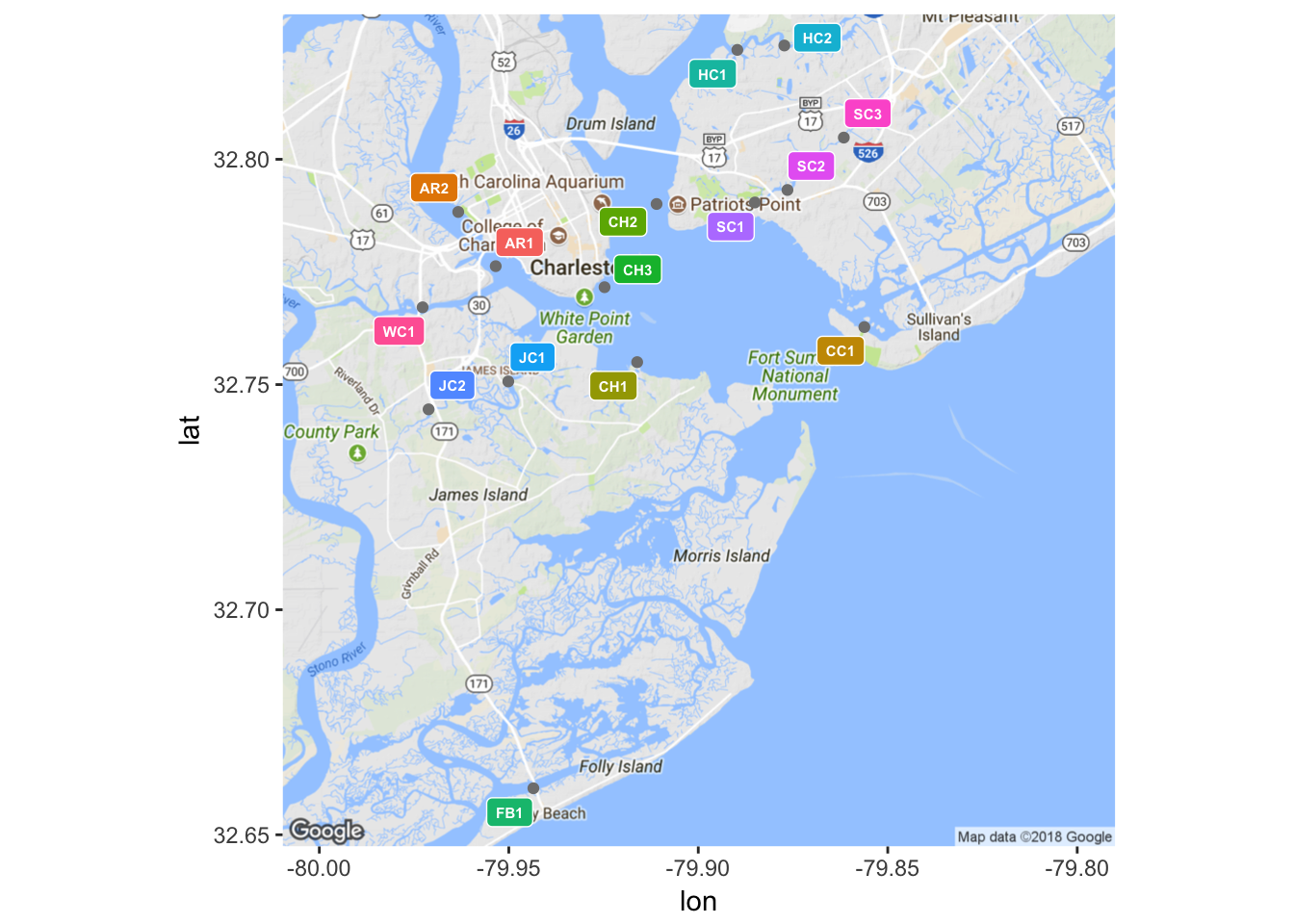
(#fig:plot_sites.2)Locations of sample sites
| ID | Description |
|---|---|
| AR1 | Ashley River |
| AR2 | Brittlebank Park |
| CC1 | Cove Creek |
| CH1 | Melton Peter Demetre Park |
| CH2 | College of Charleston Sailing |
| CH3 | Battery Beach |
| FB1 | Folly Beach Boat Landing |
| HC1 | Hobcaw Creek |
| HC2 | Hobcaw Creek |
| JC1 | James Island Creek |
| JC2 | James Island Creek |
| SC1 | Shem Creek |
| SC2 | Shem Creek |
| SC3 | Shem Creek |
| WC1 | Wappoo Cut Boat Ramp |
Modeling Intuition
Sources from coastal ecosystems literature suggest that wetland watersheds often experience a degradation in water quality after significant rainfall events [4]. The suspected mechanism driving this phenomenon is storm water runoff from impervious land surfaces surrounding a body of water. Sample sites in areas with a high percentage of impervious surface coverage are expected to be more severely impacted by rainfall events than those with relatively permeable surrounding land. The variety of surrounding landscapes among the 15 sample sites can be seen in Figure 1. Thus sample site may be a meaningful variable for predicting Enterococcus concentrations.
Similarly, the tidal stage at the time of sampling is suspected to have an impact on the concentration of Enterococcus, with ebb tides tending to be associated with higher bacteria readings than flood tides. This suspicion is grounded more in experience working in the field and exploratory data analysis than ecological literature. However, one might imagine what is occurring during ebb and flood tide while studying Figure 1 and agree that the hypothesis is reasonable. To speak in generalizations, water from the inland rivers and creeks flows out of the harbor and into the ocean during an ebb tide. Compared to ocean water, this ebb tide is relatively “dirty”, in terms of the Enterococcus metric, as it has been subjected to storm water runoff from surrounding impervious surfaces. Conversely, the ocean water that fills the harbor during a flood tide has not been polluted with runoff and thus it dilutes any of the pollutants found in the more estuarine waters. Rationalizations such as this are not meant to conjecture ecological phenomena, but rather to serve as a sanity check for later in the analysis.
Types of Missingness
Before developing and analyzing imputation methods, it is important to first consider the mechanisms behind loss of data from a study. Gelman and Hill develop several classifications of missingness, each resulting from unique “missing mechanisms” [5]. This project deals with two of Gelman and Hill’s classes of missingness: missingness that depends on the missing value itself, and missingness that depends on unobserved predictors. Of the 969 observations in the 2013-2015 data set, 140 (~15%) are censored and 28 (~3%) are missing.
Missingness that depends on the missing value itself has been referred to as “censoring” thus far. Censoring is a sub-class of missing, as the missingness itself is determined by whether or not the value is within a certain interval, which in this case is \((0,10)\). There is information to be gained from censored values and there is risk in treating them with haste. To see the risk in mishandling censored values, consider the three logical options for dealing with censored values in the context of predictive modeling:
- Ignore censored values by removing them from the data set, then proceed with modeling these non-censored data.
- Chose an arbitrary value within the range of missingness to replace all censored values with, say \(0\) in this case.
- Develop a protocol that attempts to gain all possible information that censored values have to offer, while avoiding bias and inefficiency.
An argument will now be presented as to why the first two of these three options are not ideal, and motivate the development of possible methods to fit the criteria of option (3). For the purpose of demonstration, take a small subset of the full 2013-2015 data, specifically all samples taken at Folly Beach Boat Landing (FB1) during the 2015 sampling season.
fb1.2015 = wq.data[(site == "FB1" & grepl("2015",date)),]Now, in order to make meaningful comparisons, the response variable, Enterococcus, will be replaced with values from a deterministic equation in precipitation, tide, and sample site. In other words, the values of precipitation, tide, and sample site present in fb1.2015 will deterministically generate artificial Enterococcus observations according to the following equation.
\[ \vec{Y}_i = {\bf X}_{i\times j}\vec{\beta}_j\] \[ i \in [1,25], \space j \in [1,4]\]
Here \(\vec{Y}\) is a vector of artificial observations, \({\bf X}\) is a design matrix corresponding to values of the predictor variables, and \(\vec{\beta}\) is a vector of parameter coefficients. Note that the columns of \({\bf X}\) correspond to the equation’s intercept, the values of precipitation in the past 72 hours, a dummy variable for the 2-stage tide factor, and a dummy variable for sample site. It is somewhat redundant to include this dummy variable for sample site, since in this case the only sample site is FB1, but it will be kept to remain consistent with later conventions. Lastly, although a negative value for the response variable is meaningless in reality, Enterococcus will be allowed below \(0\) for sake of argument.
\[ \mathbf{X} = \left[\begin{matrix} 1 & 0.14 & 0 & 1\\ 1 & 0.00 & 0 & 1\\ 1 & 1.01 & 1 & 1\\ \vdots & \vdots & \vdots & \vdots\\ 1 & 0.00 & 1 & 1 \end{matrix}\right] \]
\[ \vec{\beta} = \left[\begin{array} {rrr} 10.00\\ 16.50\\ -1.75\\ -1.11 \end{array}\right] \]
Once \({\bf X}\) has been loaded into a matrix, and \(\vec{\beta}\) into a vector, \(\vec{Y}\) can be computed and used to replace the true Enterococcus observations. The top fifth of the resultant data frame is given below.
| date | site | ent | pre | tide | fix | Y | |
|---|---|---|---|---|---|---|---|
| 499 | 10/28/2015 | FB1 | 98 | 0.14 | ebb | fixed | 11.200 |
| 512 | 10/21/2015 | FB1 | 41 | 0.00 | ebb | fixed | 8.890 |
| 527 | 10/14/2015 | FB1 | 10 | 1.01 | flood | fixed | 23.805 |
| 555 | 09/23/2015 | FB1 | 63 | 0.00 | ebb | fixed | 8.890 |
| 581 | 09/09/2015 | FB1 | 63 | 1.13 | ebb | fixed | 27.535 |
| 596 | 09/02/2015 | FB1 | 10 | 3.46 | flood | fixed | 64.230 |
Now consider excluding all censored observations from the model. This would amount to grouping the data by value of \(\vec{Y}_i\), specifically if \(\vec{Y}_i <10\). This grouping can be accomplished with a single command.
fb1.2015.cens = fb1.2015[fb1.2015$Y > 10,]From this abbreviated data frame, a model can be built to observe the effects of discarding censored observations. Information such as p-values and t-test statistics will be omitted, as they are meaningless when fitting a model to deterministic data.
cens.mod = glm(Y ~ pre + tide, data = fb1.2015.cens)| term | estimate |
|---|---|
| (Intercept) | 8.89 |
| pre | 16.50 |
| tideflood | -1.75 |
So, the model made from ignoring censored data correctly identified the underlying parameters of the generating model (note that the intercept coefficient is \(10.00 - 1.11 = 8.89\), or the sum of the intercept and sample site coefficients in \(\vec{\beta}\)). However, this scenario is not ideal, as it has shielded the interval \((0,10)\) from being included in the model, leading to a model that would incorrectly predict ~15% of the data.
To see why picking arbitrary values for censored observations should be avoided, take the data set formed by replacing all \(\vec{Y}_i <10\) with \(0\), and the resultant model.
fb1.2015.zero = fb1.2015
fb1.2015.zero[(fb1.2015.zero$Y < 10),7] = 0
zero.mod = glm(Y ~ pre + tide, data = fb1.2015.zero)| term | estimate |
|---|---|
| (Intercept) | 3.308305 |
| pre | 19.609164 |
| tideflood | -2.110561 |
Hence, the parameter estimates of the model can be corrupted by replacing censored observations with arbitrary constant values from within the interval of censoring. With these two cautions in mind, it is sensible to search for other ways of dealing with censored data. A collection of such methods will be considered later in this paper.
Missingness that depends on unobserved predictors is the second, and much less prevalent, type of missingness present in these data. Gelman and Hill describe this type of missingness as that which results from variables not observed and thus not possible to include in the model. In this case, the unobserved variable responsible for missingness is the event of dangerous weather during the sampling window that prevents samples from being taken at some or all of the fifteen sample sites in a given week. As in the censored case, there are a few general courses of action to take with missing data. For the same reasons as presented above, ignoring or arbitrarily replacing missing values are approaches that should be avoided. An available method for dealing with missing observations is to build a model from all non-missing observations, and then use that model to predict missing observations based on their associated values of the predictor variables. This method has model-stabilizing characteristics, but does not yield any new information. A simple proof of this claim is as follows.
Consider the case of simple linear regression on a data set with \(n\) total observations, of which \(m\) are missing. The model made from all \(n-m\) non-missing observations will be of the usual form \(E(y_i) = {\beta_0}+\beta_1x_i\) for all \(1 \le i \le n-m\), where \(\beta_0\) and \(\beta_1\) are estimated by minimizing
\[SSE_0 = \sum_{i=1}^{n-m} (y_i - \hat{y_i})^2 = \sum_{i=1}^{n-m}(y_i-(\hat{\beta_0}+\hat{\beta_1}x_i))^2\] Solving the least squares equations for each of \(\hat{\beta_0}\) and \(\hat{\beta_1}\) gives
\[ \hat{\beta_0} = \bar{y}-\hat{\beta_1}\bar{x} \]
\[ \hat{\beta_1} = \frac{S_{xy}}{S_{xx}} = \frac{\sum_{i=1}^{n-m} (x_i-\bar{x})(y_i-\bar{y})}{\sum_{i=1}^{n-m} (x_i-\bar{x})^2} \]
Let \(\vec{y^*}\) be the set of predictions \(y^*_j\), for all \(1 \le j \le m\), obtained from this model using the \(m\) values of \(\vec{x}\) associated with missing observations. Label these values of \(\vec{x}\) as \(x^*_j\) for all \(1\le j \le m\). Explicitly, \(\vec{y^*} = \hat{\beta_0^*}+\hat{\beta_1}\vec{x}\)
Now, the new model made from all \(n\) observations will have parameter coefficients obtained from solving the least squares equations given by minimizing
\[SSE_1 = \sum_{k=1}^{n}(y_k-(\hat{\beta_0}+\hat{\beta_1}x_k))^2\] \[= \sum_{i=1}^{n-m}(y_i-(\hat{\beta_0}+\hat{\beta_1}x_i))^2+\sum_{j=1}^{m}(y_j^*-(\hat{\beta_0}+\hat{\beta_1}x_j^*))^2\] \[= \sum_{i=1}^{n-m}(y_i-(\hat{\beta_0}+\hat{\beta_1}x_i))^2 + 0 = \sum_{i=1}^{n-m}(y_i-(\hat{\beta_0}+\hat{\beta_1}x_i))^2 = SSE_0\]
Hence, the parameter coefficient estimates obtained by minimizing the least squares equations for \(SSE_1\) will be identical to those obtained by minimizing the least squares equations for \(SSE_0\), since \(SSE_1 = SSE_0\). Imputing missing values in this manner would only serve to introduce data points that are exactly on the regression line.
Now that it has been established that care should be taken when imputing missing and censored values, the criteria for what makes some imputation methods better than others should be discussed.
Method Comparison Criteria
As the title suggests, a main goal of this paper is to compare the effects of different imputation methods on a final predictive model for Enterococcus. There are several criteria that could be used to compare methods, but the following metrics will be reported and discussed.
Ability to faithfully reproduce model parameters: When a test data set is produced deterministically according to an equation with known parameters, and that test data set is artificially made to have various degrees of censoring and missingness, does the imputation method produce a data set upon which a model can be built that closely resembles the underlying deterministic equation?
Predictive Bias: Does the resultant data set lead to inference that is, on average, overstating or understating reality? In the context of modeling, is it the case that the expected value of Enterococcus given by a certain model is equal to the true value of Enterococcus?
Predictive Variance: What is the variance of the difference between the prediction given by models that are built from imputed data and true values?
Convergence properties: Does the algorithm converge to a stable state? If so, does it do so quickly or after many iterations? Note for some imputation methods that rely on repeated random sampling from certain distribution, the issue of convergence is not applicable.
Computational efficiency: Is the algorithm scalable to larger data sets?
This list is not exhaustive, but it will allow for the comparison of each imputation method.
Methodology
Initial Imputation
Before visualizing and exploring the data, a preliminary attempt at imputing missing and censored values of the response variable, Enterococcus, must be made. More details will be provided in a subsequent section of this paper, but a short description of this initial imputation method is warranted here. An estimate of censored observations can be obtained by sampling from a \(Uniform(0,10)\) distribution. Missing values will be replaced with the overall mean of Enteroccocus for that particular sample site and year. Once necessary imputations are performed, a “complete” data set can be saved and used for exploratory analysis.
First, examining the first five rows of the raw data saved as a data frame named wq.data:
| date | site | ent | pre | tide | fix |
|---|---|---|---|---|---|
| 10/30/2013 | AR1 | 10 | 0.00 | flood | fixed |
| 10/30/2013 | AR2 | 213 | 1.46 | ebb | fixed |
| 10/30/2013 | CC1 | 161 | 1.46 | ebb | fixed |
| 10/30/2013 | CH1 | 135 | 1.46 | ebb | fixed |
| 10/30/2013 | CH2 | 10 | 0.02 | flood | fixed |
| 10/30/2013 | FB1 | 20 | 0.00 | ebb | fixed |
Sub-setting the wq.data data frame into complete.set, censored.set, and missing.set.
complete.set = wq.data[(ent != "--" & ent != "<10"),]
censored.set = wq.data[(ent == "<10"),]
missing.set = wq.data[(ent == "--"),]
Now samples can be taken from the \(Uniform(0,10)\) distribution.
cens.sample = ceiling(runif(length(censored.set[,1]),0,10))
censored.set[,3] = cens.sample
The task of computing appropriate means as specified above is slightly more tedious, so that code will be included in the appendix. Essentially, once data is grouped by sample site and sampling season using a similar approach as above, computing means is trivial. Finally, the separate complete.set, censored.set, and missing.set data frames can be combined back into wq.data.
wq.data = rbind(complete.set,censored.set,missing.set)The data are now prepared for exploratory analysis.
Visual Exploration
As was mentioned in the introduction, a simple hypothesis made after working in the field is that Enterococcus behaves differently depending on the tidal stage at the time of sampling. Namely, Enterococcus concentrations are thought to be higher during ebb tides than flood tides. Using R and ggplot2, the conditional density curve of Enterococcus for each tidal stage can be visualized. The following plot is called a “violin” plot for its ability to sometimes resemble the outline of a violin. Violin plots are a succinct way to compare two or more density curves.
ggplot(wq.data,aes(tide,log(ent))) + geom_violin(aes(fill=tide)) + labs(x="Tidal Stage",y="ln(Ent.)")vs.Tide-1.png)
(#fig:plot_Ln(Ent)vs.Tide)ln(Ent.) conditioned on tidal stage
Note that a natural logarithm transformation was applied to the response variable, Enterococcus. Due to its extreme variability, an untransformed Enterococcus variable cannot be easily visualized or modeled. The natural logarithm transformation will be used throughout this paper, and unless otherwise noted, both Enterococcus and \(log(Enterococcus)\) can be thought to imply \(ln(Enterococcus)\).
Another suspected phenomenon is that Enterococcus levels are expected to be higher at some sample sites than at others, all other factors adjusted for. A similar violin plot can be constructed for the density curve of Enterococcus at each sample site, as seen in Figure 3.
ggplot(wq.data,aes(site,log(ent))) + geom_violin(aes(fill=site)) + labs(x="Sample Site",y="ln(Ent.)")vs.Site-1.png)
(#fig:plot_Ln(Ent)vs.Site)ln(Ent.) conditioned on sample site
Of course, whatever effect that tidal stage may have on Enterococcus is dependent on the sampling site. The converse is also true. Since less voluminous waters are more tidal by nature, it is reasonable to expect that the smaller creeks in the bevy of sample sites will be more dramatically impacted by tidal stage than those in more open waters. Combining Figures 2 and 3 gives the conditional density curves of Enterococcus for each combination of sample site and tidal stage shown in Figure 4.
ggplot(wq.data,aes(tide,log(ent))) + geom_violin(aes(fill=site)) + labs(x="Tidal Stage",y="ln(Ent.)")vs.Tidevs.Site-1.png)
(#fig:plot_Ln(Ent)vs.Tidevs.Site)ln(Ent.) conditioned on tidal stage and sample site
Visualizing the relationship between \(ln(Ent.)\) and precipitation is slightly more complicated, as it is best considered individually for each site. In Figure 5, \(ln(Ent.)\) is plotted versus \(ln(precip.)\) and faceted by sample site.
ggplot(wq.data,aes(log(pre),log(ent))) + geom_point(aes(color=tide)) + facet_wrap(~ site)vs.ln(Precip)vs.Site-1.png)
(#fig:plot_Ln(Ent)vs.ln(Precip)vs.Site)ln(Ent.) vs. ln(Precip) for each sample site
Data for precipitation 72 hours prior to sampling was obtained from a collection of 18 National Oceanographic and Atmospheric Administration (NOAA) gauges in the Charleston area. Charleston Waterkeeper records precipitation levels for the 24 hours prior to sampling, but this window was thought to not be large enough to encompass all of the rainfall events that may affect an Enterococcus measurement. Each of the 15 sample sites was paired with the closest of NOAA’s rain gauges, and the amount of precipitation in inches was retroactively appended to the data set. Unfortunately, there was not complete continuity in NOAA’s records, so it was not always possible to follow this rule. In the event of a missing precipitation record for the closest gauge to a given sample site, the next closest gauge was consulted instead. Due to the need to make a decision on a case by case basis about which rain gauge to consult, this process could not have been easily automated. Ideally, each nearest rain gauge would have continuous and complete temporal coverage over the timeline of this analysis, but that was sadly not the case. Figure 6 shows a map of the locations of NOAA’s rain gauges.
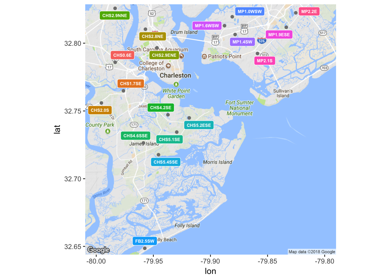
(#fig:plot_gauges)Locations of NOAA rain gauges.
Generating Test Data
To compare the effects of each imputation method, it is important to know the characteristics of the data set being used. Thus, an artificial test data set must be constructed in R using a similar approach as in the Types of Missingness section of this paper. However, here the test data set will be made to resemble the full data set with all 969 observations. The function genTestData() will be defined to generate a test data frame. The function will take in parameters in.set for the input set to be replicated, cens.limit for the limit of left censoring, and percent.missing corresponding to the percent of observations in the test data set that will artificially be made missing. Refer to the appendix for the full code behind the function. The output of the function will be saved to test.df, which will act as the data set to test each of the following imputation methods on.
test.df = genTestData(wq.data, 10, 5)Method 1: A naive approach.
The first method was introduced briefly in the Initial Imputation subsection and will be encoded in the basicImputation() function given in the appendix. The general goal of this technique is to make a preliminary attempt at imputing missing and censored values, but to keep the strategy simple to allow for meaningful comparison to more sophisticated methods later on. Specifically, censored values will be replaced with a random sample from a \(Uniform(0,10)\) distribution, and the ceiling function will be applied to ensure all values are in the domain of the natural logarithm function. Missing values in this method will be imputed with the overall mean of Enterococcus, after censored observations have been sampled. Once this is done, a model will be built from the now complete data set, and model parameters will be stored.
The model equation used here, and for each subsequent imputation method, will be as follows.
\[E(ln(Ent.)) = \beta_0 + \beta_{precip}(precip)+\beta_{flood}(flood)+\beta_{AR2}+...+\beta_{WC1}\]
This procedure will be repeated N times, where N is passed through via parameter. The result will be an \(N\times17\) data frame of model parameter estimates returned by the function. Refer to the appendix for the R code used to accomplish this.
basic.df = basicImputation(100,test.df)Method 2: Sampling from a Truncated Normal.
Here, a slightly more refined method will be employed, namely by introducing the Truncated Normal distribution to sample replacement values for censored observations. The truncated normal distribution is more tightly centered about its mean than the uniform distribution, so overall, the samples used to replace censored values will be expected to have a lower overall variability than in the previous method. Using the truncnorm package in R, and in particular the function rtruncnorm(), truncated normal random variables can be easily generated.
In pursuit of stable estimates of model parameters over many simulations, missing values will be imputed by the prediction given by a model built from all non-missing data, after censored observations have been sampled from a truncated normal distribution. It was shown previously in the Types of Missingness section that doing so has no effect on the estimate of model parameter coefficients, because no “new information” is obtained.
The algorithm for implementing this method will proceed similarly to Method 1. The data will be separated into a complete set, a censored set, and a missing set. For each of the N iterations, censored values will be sampled from a truncated normal distribution, and added back to the complete set. Then, a model will be built from all non-missing values and used to predict missing observations. Finally, these newly predicted values will be added back to the complete set and a final model will be built on this complete set. At each step of the simulation, estimates of model parameter coefficients will be stored. These steps are performed by the function truncNormSampler(), and the full code is given in the appendix.
The parameters accepted by truncNormSampler() are N for simulation size, in.set for the test data set, t.a for the left bound of truncation, t.b for the right bound of truncation, t.mean for the mean of the truncated normal, and t.sd for the standard deviation of the truncated normal. A \(N\times17\) data frame of parameter coefficient estimates is returned by the function.
truncSamp.df <- truncNormSampler(100,test.df)Method 3: Imputation from the expected value of a Truncated Normal
The third and final method will again involve the truncated normal distribution, but instead of randomly sampling from a truncated normal random variable, censored values will be replaced with its expected value. More precisely, if \(Y\) is a random variable corresponding to the natural logarithm of Enterococcus, then the following assumptions are being made.
\[ Y \sim logNormal(\mu,\sigma^2) \implies ln(Y) \sim Normal(\mu,\sigma^2) \]
Note \(ln(Y)\) is the variable to be truncated below some constant \(a\) and above some constant \(b\). Ultimately, \(E[ln(Y)|a<ln(Y)<b]\) is desired. Standardizing,
\[ E[ln(Y)|a<ln(Y)<b] = E[(\frac{ln(Y)-\mu}{\sigma}+\frac{\mu}{\sigma})\sigma | \frac{a-\mu}{\sigma}<\frac{ln(Y)-\mu}{\sigma}<\frac{b-\mu}{\sigma}]. \] Letting \(Z\) denote a standard normal random variable, \(\alpha = \frac{a-\mu}{\sigma}\), and \(\beta=\frac{b-\mu}{\sigma}\), this expected value can be simplified to
\[ \sigma E[Z|\alpha<Z<\beta]+\mu. \]
From the definition of a truncated normal random variable,
\[ E[Z|\alpha<Z<\beta] = \int_{\alpha}^{\beta}z{\frac{\phi(z)}{\Phi(\beta)-\Phi(\alpha)}}dz = \frac{\int_{\alpha}^{\beta}z\phi(z)dz}{\Phi(\beta)-\Phi(\alpha)}, \] where \(\phi(z)\) and \(\Phi(z)\) denote the probability density function and cumulative distribution function of \(Z\) respectively. Considering the numerator of this last fraction,
\[\int_{\alpha}^{\beta}z\phi(z)dz=\int_{\alpha}^{\beta}z\frac{1}{\sqrt{2\pi}}e^{-\frac{1}{2}z^2}dz,\] and letting \(w = \frac{1}{2}z^2\), the following observations can be made.
\[ dw = zdz \] \[ z=\alpha \implies w= \frac{1}{2}\alpha^2 \] \[ z = \beta \implies w = \frac{1}{2}\beta^2 \]
As a result,
\[ \int_{\alpha}^{\beta}z\phi(z)dz=\int_{\frac{1}{2}\alpha^2}^{\frac{1}{2}\beta^2} \frac{1}{\sqrt{2\pi}}e^{-w}dw = \frac{1}{\sqrt{2\pi}}[e^{-\frac{1}{2}\alpha^2}-e^{-\frac{1}{2}\beta^2}] = \phi(\alpha)-\phi(\beta) \]
Thus \(E[Z|\alpha<Z<\beta]= \frac{\phi(\alpha)-\phi(\beta)}{\Phi(\beta)-\Phi(\alpha)}\), and finally
\[ E[ln(Y)|a<ln(Y)<b] = \mu+\sigma{\frac{\phi(\frac{a-\mu}{\sigma})-\phi(\frac{b-\mu}{\sigma})}{\Phi(\frac{b-\mu}{\sigma})-\Phi(\frac{a-\mu}{\sigma})}}. \]
For the purposes of imputing censored values in this context, \(Y\) will be restricted to be between \(0\) and \(10\) and therefore \(ln(Y)\) will have support \((-\infty,ln(10))\). When letting \(a = -\infty\) and \(b = ln(10)\), the above equation simplifies to
\[ E(ln(Y)|0<ln(Y)<ln(10))=\mu-\sigma{\frac{\phi(\frac{ln(10)-\mu}{\sigma})}{\Phi(\frac{ln(10)-\mu}{\sigma})}}. \]
To compute this expected value, estimates for \(\mu\) and \(\sigma\) must be obtained. The approach that will be taken here is to build a starter model from all non-censored and non-missing values, then use that starter model to obtain initial estimates for \(\mu\) and \(\sigma\). More formally, each censored observation \(Y_c\), will be replaced by
\[ Y^* = \hat{\mu}-\hat{\sigma}{\frac{\phi(\frac{ln(10)-\hat{\mu}}{\hat{\sigma}})}{\Phi(\frac{ln(10)-\hat{\mu}}{\hat{\sigma}})}}, \]
where \(\hat{\mu}={\bf X}_{i\times j}\vec{\beta}_j\), the prediction given by the starter model for the set of predictor variable values associated with \(Y_c\), and \(\hat{\sigma}=\frac{\sum(\hat{Y_i}-Y_i)^2}{n^*}\), the mean squared error of the starter model, where \(n^*\) is the number of complete observations in the data set.
Missing values will then be predicted by the model made from all non-missing data, and then added back to the complete data set. Then a final model will be built from this full data set, and the models parameter coefficient estimates will be stored. The function truncNormExpVal() performs these steps, and full code for the function is included in the appendix. Only the parameters N for simulation size, and in.set for the test data set are needed.
truncExp.df <- truncNormExpVal(100,test.df)Modeling
Once the results from each imputation algorithm are compared, the modeling phase of this project may begin. Of the many possibilities for model choices, two types of models will be pursued: those that model \(ln(Enterococcus)\) as a continuous numeric random variable, and those that model the probability of Enterococcus exceeding the state-mandated safety threshold for recreational waters.
Continuous numeric outcome: A general linear model will be used to model \(ln(Enterococcus)\) in this case. The standard assumptions that the model errors, \(\epsilon_i \stackrel{iid}{\sim} Normal(0,\sigma^2)\) will be checked and attention will be paid to the significance of each parameter coefficient estimate as well as the coefficient of determination for the model.
Binary categorical outcome: Here, logistic regression will be used to estimate the probability of Enterococcus exceeding a certain threshold. Such an estimate may be favorable over the continuous numeric case, as it has easy interpretability in terms of the risk of coming in contact with water from a certain waterway under a given set of conditions. The assumption that each \(Y_i \stackrel{ind}{\sim} Binomial(n_i,\pi_i)\) will be evaluated as well.
The results of each modeling attempt will be analyzed and used to determine what the best model of Enteroccocus concentrations is for the purposes of this study.
Results
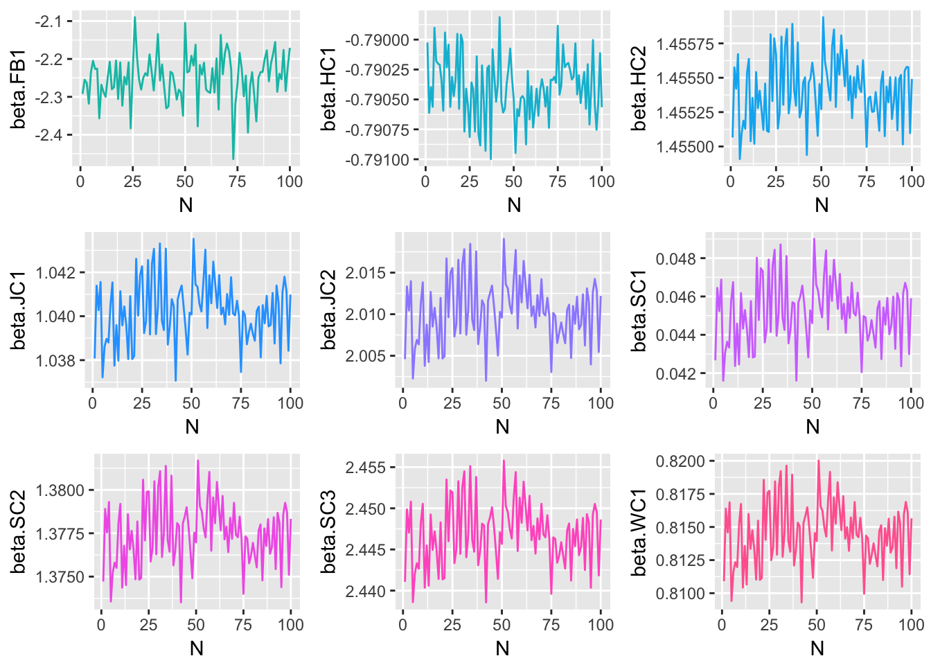
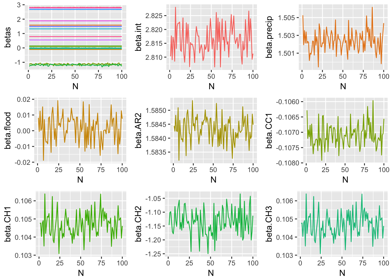
Since each of the three methods considered were iterative processes, and parameter estimates were obtained at each step of the iteration, one way to track the behavior of each method is to plot the estimate for each model parameter at each \(n=1,2,...,N\). The following plots display the estimate of each model coefficient at each step of the simulation. By themselves, these plots are not very meaningful, but when they are viewed in conjunction with an understanding of the criteria established in the section of this paper, and the true parameter coefficient values, used in the genTestData() function.
Method 1 Simulation Results

Method 2 Simulation Results
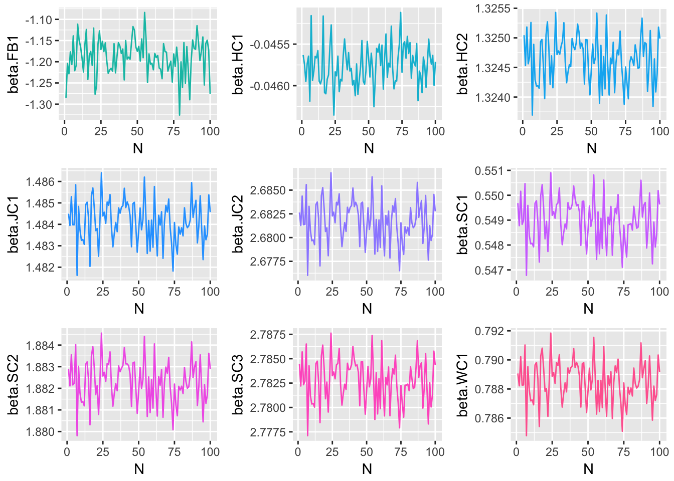
Method 3 Simulation Results
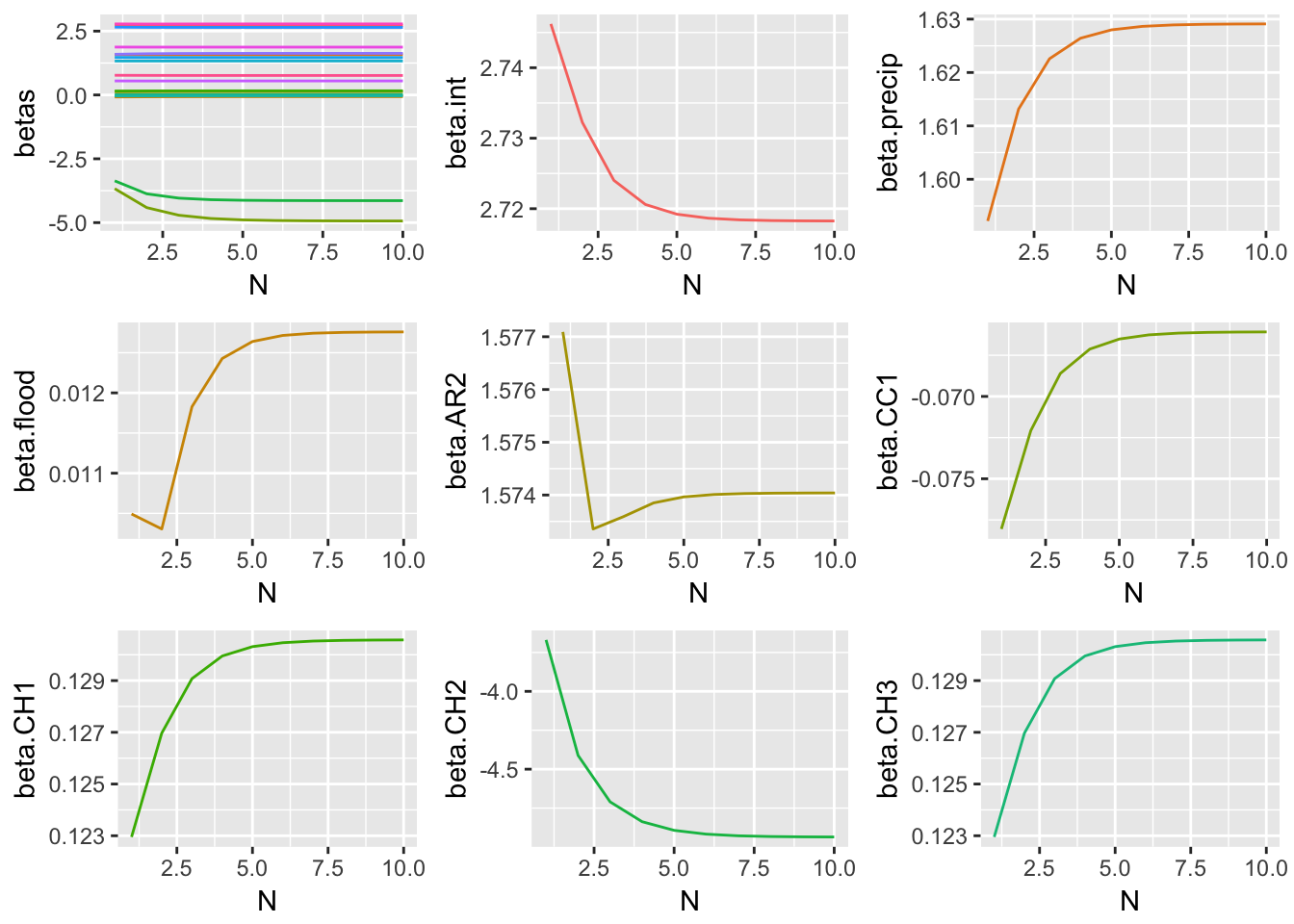
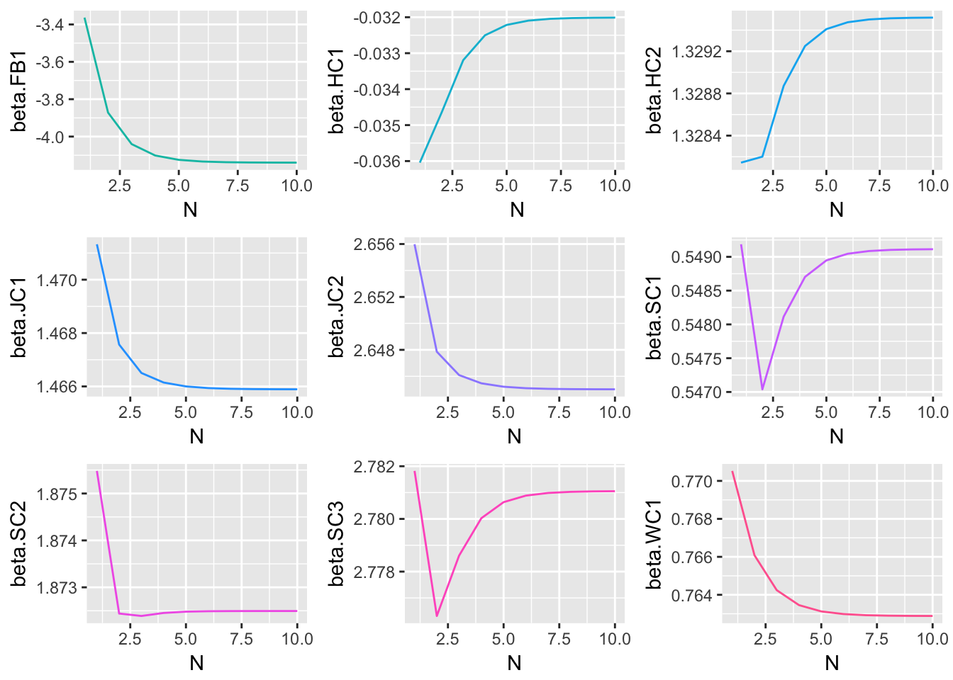
These graphical representations of the simulations performed for each imputation method can be supplemented with numerical results as well. Specifically, the absolute difference between the estimates of model parameter coefficients and true coefficients for each imputation method are documented. What follows is a summary containing the sum of these coefficient errors, the predictive bias, and the predictive variance.
| Coeff. | True | M1 Med. | M1 Err. | M2 Med. | M2 Err. | M3 Final | M3 Err. |
|---|---|---|---|---|---|---|---|
| (Intercept) | 2.8 | 3.804 | 1.004 | 2.816 | 0.016 | 2.718 | 0.082 |
| pre | 1.5 | 1.401 | 0.099 | 1.502 | 0.002 | 1.629 | 0.129 |
| flood | -1.75 | 0.118 | 1.868 | 0.002 | 1.752 | 0.013 | 1.763 |
| AR2 | 1.6 | 1.191 | 0.409 | 1.584 | 0.016 | 1.574 | 0.026 |
| CC1 | -0.1 | -0.728 | 0.628 | -0.107 | 0.007 | -0.066 | 0.034 |
| CH1 | 0.1 | -0.123 | 0.223 | 0.105 | 0.005 | 0.131 | 0.031 |
| CH2 | -0.95 | -2.042 | 1.092 | -1.137 | 0.187 | -4.936 | 3.986 |
| CH3 | 0.14 | -0.318 | 0.458 | 0.133 | 0.007 | 0.162 | 0.022 |
| FB1 | -1.11 | -2.243 | 1.133 | -1.185 | 0.075 | -4.139 | 3.029 |
| HC1 | -0.04 | -0.79 | 0.75 | -0.046 | 0.006 | -0.032 | 0.008 |
| HC2 | 1.34 | 1.455 | 0.115 | 1.325 | 0.015 | 1.33 | 0.01 |
| JC1 | 1.5 | 1.04 | 0.46 | 1.484 | 0.016 | 1.466 | 0.034 |
| JC2 | 2.7 | 2.01 | 0.69 | 2.682 | 0.018 | 2.645 | 0.055 |
| SC1 | 0.56 | 0.045 | 0.515 | 0.549 | 0.011 | 0.549 | 0.011 |
| SC2 | 1.9 | 1.378 | 0.522 | 1.882 | 0.018 | 1.872 | 0.028 |
| SC3 | 2.8 | 2.447 | 0.353 | 2.783 | 0.017 | 2.781 | 0.019 |
| WC1 | 0.8 | 0.815 | 0.015 | 0.788 | 0.012 | 0.763 | 0.037 |
| Total Abs. Coeff. Error | Predictive Bias | Predictive Variance | |
|---|---|---|---|
| Method 1 | 10.334 | 0.448 | 0.135 |
| Method 2 | 2.180 | -0.010 | 0.002 |
| Method 3 | 9.304 | -0.492 | 1.567 |
The above results suggest that of the three imputation methods considered, Method 2 is best able to faithfully replicate underlying model parameters, while minimizing predictive bias and variance. Therefore Method 2 will be used to perform imputation of missing and censored values before modeling.
model.df <- truncNormSampler(1,wq.data,ret = "data")Modeling
Now that imputation has been performed according to Method 2, a model of \(ln(Ent.)\) as a continuous numeric random variable in terms of precipitation in the past 72 hours, tidal stage, and sample site can be built.
model.glm = glm(log(ent) ~ pre + tide + site, data = model.df)Below is a summary of the model characteristics for model.glm as well as appropriate plots for verifying regression assumptions.
library(ggfortify)
autoplot(model.glm)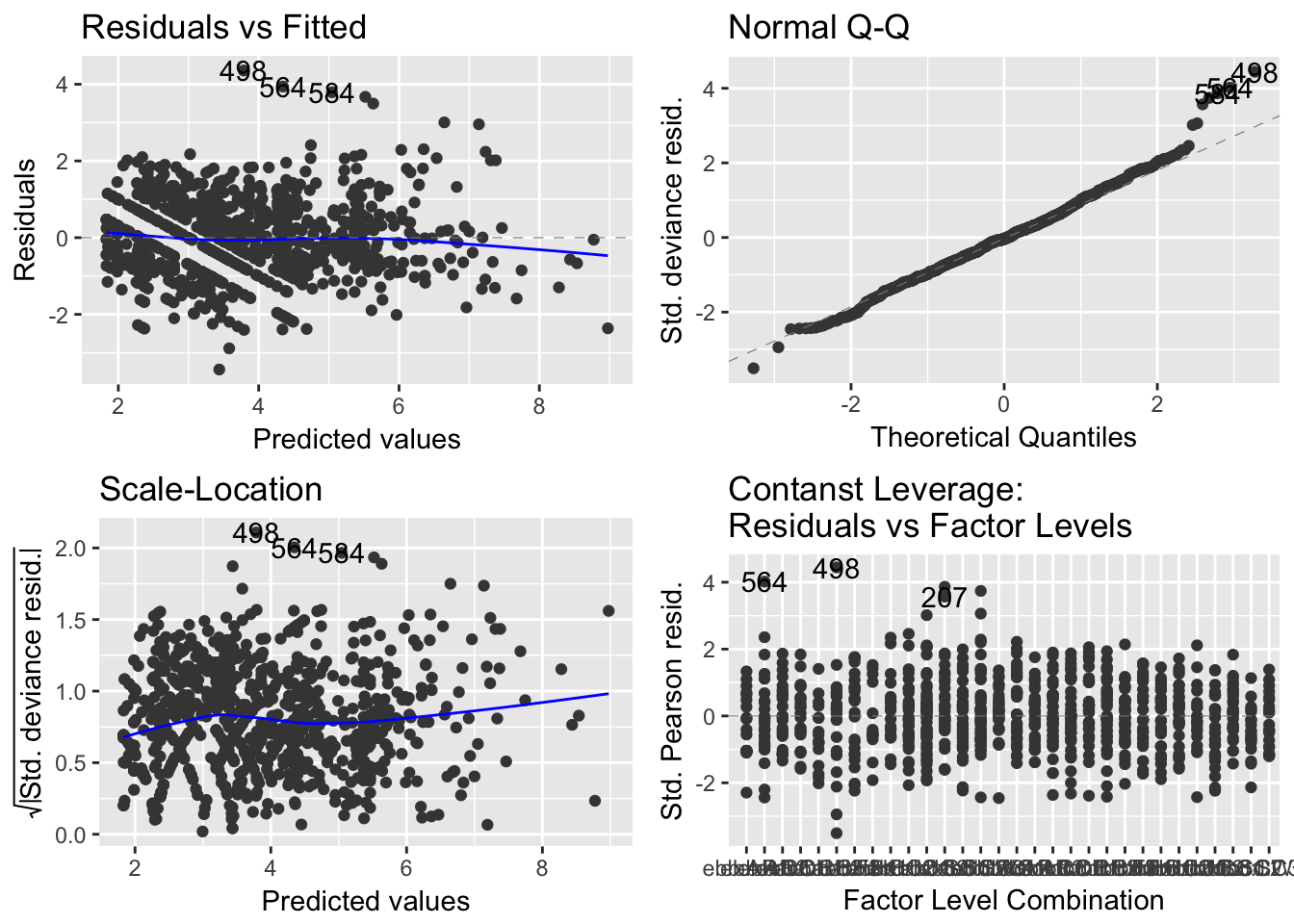
(#fig:model.1.2)GLM Residual Analysis
It can be seen from Figure 8 that while the spread of the residuals divided by standard residuals remains roughly constant for each value of the precipitation variable, there is a downward pattern that may suggest there are trends affecting the relationship between precipitation and \(ln(Enterococcus)\) that are not explained in the model.
res.glm = model.glm$residuals
stdresid.glm = rstandard(model.glm)
stdres.vs.precip = as.data.frame(cbind((res.glm/stdresid.glm),
    model.glm$data$pre))
colnames(stdres.vs.precip) = c("Res.StdRes", "Precip")
ggplot(data = stdres.vs.precip, aes(y = Res.StdRes, x = Precip)) +
    geom_point() + ylab("Residuals/Standardized Residuals") +
    xlab("Precipitation") + geom_smooth()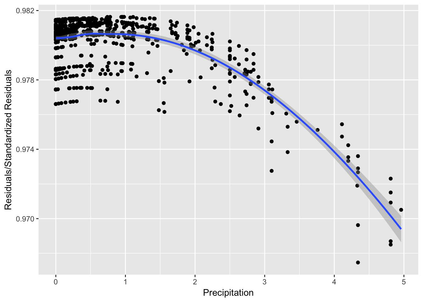
Figure 1: Precipitation vs. Residuals/StdResiduals
kable(summary(model.glm)$coeff, digits = 3, caption = "GLM Results")| Estimate | Std. Error | t value | Pr(>|t|) | |
|---|---|---|---|---|
| (Intercept) | 3.324 | 0.135 | 24.579 | 0.000 |
| pre | 0.708 | 0.036 | 19.889 | 0.000 |
| tideflood | -1.066 | 0.067 | -15.825 | 0.000 |
| siteAR2 | 1.016 | 0.175 | 5.814 | 0.000 |
| siteCC1 | 0.112 | 0.176 | 0.636 | 0.525 |
| siteCH1 | 0.021 | 0.174 | 0.120 | 0.904 |
| siteCH2 | -0.272 | 0.182 | -1.499 | 0.134 |
| siteCH3 | 0.115 | 0.174 | 0.657 | 0.511 |
| siteFB1 | -0.426 | 0.174 | -2.441 | 0.015 |
| siteHC1 | 0.162 | 0.196 | 0.829 | 0.407 |
| siteHC2 | 0.937 | 0.189 | 4.965 | 0.000 |
| siteJC1 | 0.946 | 0.175 | 5.402 | 0.000 |
| siteJC2 | 2.044 | 0.176 | 11.580 | 0.000 |
| siteSC1 | 0.538 | 0.175 | 3.078 | 0.002 |
| siteSC2 | 1.068 | 0.175 | 6.110 | 0.000 |
| siteSC3 | 2.139 | 0.176 | 12.149 | 0.000 |
| siteWC1 | 0.460 | 0.188 | 2.445 | 0.015 |
Also of interest is a model relating the exceedence of Enterococcus beyond a certain predetermined safety threshold. A binary variable for whether or not Enterococcus exceeds this safety limit can be retroactively created and modeled in terms of the original data set.
safety.lim = 40
exceed = as.numeric(model.df[, 3] > safety.lim)
model.logist = glm(exceed ~ pre + tide + site, data = model.df,
    family = binomial())
Finally, a summary of the model characteristics for model.logist and regression assumption diagnostic plots are given below.
kable(summary(model.logist)$coeff, digits = 3, caption = "Logistic Regression Results")| Estimate | Std. Error | z value | Pr(>|z|) | |
|---|---|---|---|---|
| (Intercept) | -0.469 | 0.347 | -1.351 | 0.177 |
| pre | 1.383 | 0.162 | 8.553 | 0.000 |
| tideflood | -1.921 | 0.188 | -10.226 | 0.000 |
| siteAR2 | 1.803 | 0.452 | 3.988 | 0.000 |
| siteCC1 | -0.171 | 0.467 | -0.366 | 0.714 |
| siteCH1 | -0.143 | 0.468 | -0.305 | 0.761 |
| siteCH2 | -0.212 | 0.499 | -0.424 | 0.671 |
| siteCH3 | 0.155 | 0.458 | 0.339 | 0.735 |
| siteFB1 | -0.762 | 0.492 | -1.547 | 0.122 |
| siteHC1 | 0.530 | 0.505 | 1.049 | 0.294 |
| siteHC2 | 2.030 | 0.485 | 4.186 | 0.000 |
| siteJC1 | 1.934 | 0.463 | 4.179 | 0.000 |
| siteJC2 | 4.080 | 0.810 | 5.039 | 0.000 |
| siteSC1 | 0.868 | 0.444 | 1.956 | 0.050 |
| siteSC2 | 1.877 | 0.457 | 4.110 | 0.000 |
| siteSC3 | 3.595 | 0.637 | 5.647 | 0.000 |
| siteWC1 | 0.902 | 0.474 | 1.904 | 0.057 |
Conclusions
Imputation Methods
While there were noticeable differences in the results produced by each imputation method, all three methods performed fairly well. Of the three methods considered, Method 2 performed best in terms of minimizing the overall absolute value errors of the parameter coefficient estimates, the predictive bias, and the predictive variance of the resultant model. In methods 1 and 2, the issue of convergence was not relevant, since both rely on random sampling at each iteration of the simulation. Method 3 did converge to a stable set of model parameter coefficient estimates after roughly \(N=10\) simulations, but convergence was not considered as important as the first three criteria mentioned. Method 2 was therefore chosen to perform imputation in preparation for the modeling phase.
Modeling
Modeling \(ln(Enterococcus)\) as a continuous numeric random variable in terms of precipitation, tidal stage, and sample site was achieved with adequate success. Splitting the 15-level sample site factor variable into 14 dummy variables for this model may have been the reason that four of them were not significant at any reasonable significance level. However, the main variables of interest, precipitation and tide, were highly significant. In terms of regression assumptions, this model did not display any flagrant violations of the distributional assumptions for the model errors. Even after the natural logarithm transformation, there were still outliers in the distribution of water quality - a testament to the high variability of Enterococcus in the field. These outliers were not influential enough to severely alter the model, so it was not necessary to consider removing them from this analysis.
The results from modeling component of this project suggest that overall, increased precipitation in the past 72 hours has a detrimental effect on water quality around Charleston. Similarly, ebb tides tend to feature higher bacteria levels than flood tides. Both the precipitation and tidal stage variables were highly significant in the general linear model. The sample sites that are the most prone to high bacteria counts, such as those in Shem Creek and James Island Creek, have significant coefficient estimates in the general linear model, suggesting that these sites have significantly higher bacteria levels on average. Sample sites that do not have significant coefficients in the general linear model are those that also rarely feature dangerously high bacteria levels. The model suggests that these sites, such as Hobcaw Creek and Charleston Harbor, are not expected to have significantly different bacteria levels, adjusting for precipitation and tidal stage.
Compared with the continuous numeric model, using logistic regression to model the exceedance of Enterococcus beyond a certain safety limit was not as successful. In the logistic model, there were several non-significant coefficient estimates, suggesting the model’s credibility may be doubtful. In light of this and the fact that it is generally more desirable to be able to predict Enterococcus as a continuous numeric variable than an binary one, it is not recommended that the logistic model be used in practice to model Enterococcus concentrations. This leaves the continuous numeric model as the chosen model for future use.
Discussion
Critiques
There are several areas in which this project could be improved. Below is a brief list of critiques that are acknowledged.
This project relied on data from the 2013-2015 sampling seasons. Data for the 2016 season were available at the time of this writing, but were not included because work on this project began before these most recent observations were released. In the interest of time, the analyses presented here were not redone to incorporate 2016 data, but this could be a future area of improvement.
The process of associating NOAA rain gauges with Charleston Waterkeeper Sample sites, as described on pg. 17, invited the possibility of human error. Ideally, there would be a more standardized way to assign precipitation measurements to Enterococcus observations.
While the chosen model for Enterococcus assumed a linear relation between \(ln(Ent.)\) and precipitation, controlling for both tidal stage and sample site, there were some instances of slight violations of this assumption, as evidenced by Figure 5.
Decisions regarding the procedural details of each imputation method were more grounded in intuition than statistical literature. If time had permitted, the literature could have been more thoroughly mined for studies that considered similar methods.
This project was almost entirely reliant upon
Rprogramming. As with most extensive programming endeavors, there are ample opportunities for improving efficiency and eliminating any bugs that may not be immediately visible. Serious effort was addressed to both of these concerns, as well as to the desire to make this project fully reproducible by using R Markdown and posting code and data to the website for this project.Because of extreme weather events contained in the 2013-2015 records, such as the historic rain that occured in October of 2015, there are outliers in both the \(Enterococcus\) and precipitation variables. The final general linear model would benefit from outlier analysis and possibly outlier removal, since the intention of the model is not to predict bacteria counts under such extreme and rare conditions.
In light of these drawbacks, the final model built during this project can be immediately useful to both Charleston Waterkeeper and those who would like more information about the expected safety of recreational sites in the Charleston are under certain conditions. Additionally, there is a possibility that the imputation methods developed and analyzed here may be applicable to future studies.
The last component of this project was to encode the results from this paper into an interactive web application that can be used to predict the hazard associated with recreation at each of the fifteen sample sites in this study based on a certain set of environmental conditions specified by inches of rainfall in the past 72 hours and tidal stage at the time of recreation. Since this project will be finished in time for the beginning of the 2017 sampling season, the interactive water quality model that came from this analysis can be used by Charleston Waterkeeper to better inform the public about expected risks from recreation. To access the interactive water quality model, visit .
References
The Riverkeepers: Two Activists Fight to Reclaim Our Environment as a Basic Human Right by John Cronin and Robert F. Kennedy Jr.
R Studio. rmarkdown.rstudio.com.
Carmack, Cheryl & Wunderly, Andrew. Charleston Waterkeeper. Recreational Water Quality Monitoring Program Quality Assurance Project Plan. 2015.
Holland, A.Frederick, Denise M. Sanger, Christopher P. Gawle, Scott B. Lerberg, Marielis Sexto Santiago, George H.m Riekerk, Lynn E. Zimmerman, and Geoffrey I. Scott. “Linkages between Tidal Creek Ecosystems and the Landscape and Demographic Attributes of Their Watersheds.” Journal of Experimental Marine Biology and Ecology 298.2 (2004): 151-78. Web.
Gelman, Andrew, and Jennifer Hill. Data Analysis Using Regression and Multilevel/hierarchical Models. 1st ed. Cambridge: Cambridge UP, 2007. Print.
This research was supported financially by the University of South Carolina’s Magellan Scholars grant. Thank you to the University for this support and to the Magellan Scholars program for continued feedback and advice.
Appendices
Please refer to https://carter-allen.github.io for supporting materials and the interactive application built with the modeling results from this project.
Data
SortedCensoredAndMissing.txt: https://carter-allen.github.io/SortedCensoredAndMissing.txtSampledFullWaterQualityData.txt: https://carter-allen.github.io/SampledFullWaterQualityData.txtSiteLocations.txt: https://carter-allen.github.io/SiteLocations.txtSiteDescriptions.txt: https://carter-allen.github.io/SiteDescriptions.txtGaugeLocations.txt: https://carter-allen.github.io/GaugeLocations.txtModelData.txt: https://carter-allen.github.io/ModelData.txt
Code
Thesis.rmd: https://carter-allen.github.io/Thesis.rmd